Short pulse modelling in PPD

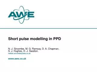
1. Short pulse modelling in PPD N. J. Sircombe, M. G. Ramsay, D. A. Chapman, S. J. Hughes, D. J. Swatton. nathan.sircombe@awe.co.uk www.awe.co.uk

2. Outline • Background • Short pulse LPI • Transport • Plans for short pulse modelling

3. Background • The twin petawatt arms on ORION will provide a means to heat matter to extreme temperatures and allow us to study its properties. • The mechanisms by which the short pulse laser delivers its energy, how this energy is distributed and how it is transported into the material are complex and interdependent.

4. Background • Currently there is a reliance on a number of empirical relations, which may be limited to a specific target configuration or laser system. • A more predictive modelling capability will help us to… • Understand, challenge or support these assumptions • Optimise experiments to make the best use of ORION’s available short-pulse capability. • There are clear similarities between the problems faced in predicting the outcome of full-scale ORION experiments and developing a fast ignition point design

5. Short pulse LPI • Modelling interaction of SP laser in • Planar targets • Variety of plasma profiles, target angles • Cone geometry • Effect of low-density cone fill • Effect of ‘missing’ cone tip • Using PIC codes and direct Vlasov solvers • CCPP PIC code – EPOCH • Developed by C. S. Brady (CFSA Warwick) • Direct, 2D, Vlasov – VALIS • Developed with T. D. Arber (CFSA Warwick)

6. Hot electron generation in planar targets • Characterise energy spectrum of hot electrons in experiments fielded on Omega • To produce radiographic source from bremsstrahlung • With and without a long-pulse created ‘pre plasma’ • Intended to improve absorption and generation of hot electrons • …but low density pre-plasma generates very high energy electrons • Potential problem for FI (e.g. foam filled cones, fuel ‘jets’ entering the cone etc.) • Bremsstrahlung radiation can be modelled using EPOCH particle probe data as a source in MCNPx

7. 90o 0o -90o 0 100MeV 200 2D ‘Cone’ Geometries • In a full 2D cone geometry, the presence of a long scale length pre-plasma: • allows more energy to be coupled into hot electrons • produces higher energy electrons • produces a more divergent beam • creates a larger effective hot electron source, as the beam is refracted. • If the short pulse laser misses the cone tip the pre-plasma has a detrimental effect • Produces a hot electron beam which is divergent • originates over a larger area • not directed at the assembled fuel.

8. VALIS • 2D2P Direct Vlasov Solver • Explicit, Conservative, Split scheme using PPM advection • Laser boundaries for LPI • Domain decomposition over 4D (2D2P) phase space • N.J. Sircombe and T.D. Arber, J. Comp. Phys. 228, 4773, (2009)

9. Hot electrons from short scale length plasmas • 500nc, 3.5 micron scale length plasma ramp • 1.37e20W/cm2 from LH boundary • System size • 80 microns in space, +/- 24bg in momentum • (nx, npx, npy) = (8192, 200, 220) • Estimate ThotUsing fit to Boltzmann distribution over three energy ranges* • [0.1, 1), [1,5) and [5,10] MeV • ‘Head’ of electron ‘beam’ not well described by Boltzmann dist. * Not an ideal solution! see M. Sherlock PoP (2009)

10. (x,ux) phase space (immobile ions) t=226fs t=226fs t=76fs ux -32 -20 -40 0 40 -20 -32 x x x • Thot peaks and falls • 7.3 MeV at 200fs, 1.5MeV at 400fs • Apparent ‘steady state’ by 200fs

11. Mobile Ions t=200fs fi fe • Preliminary results with mobile ions • Profile steepening, ion acceleration at front surface • Evidence of IAW, ion trapping in pre-plasma -8 -40 0 40 -26 x x

12. Transport • Modelling hot electron transport in solid density targets using THOR II • Explicit Monte Carlo Vlasov-Fokker-Planck solver in 2D3P or 3D3P • Eulerian grid • Self-consistent fields via return current argument

13. Buried Layer modelling • Range of intensities • Al layer buried at various depths in CH target • Lee-More resistivity model for metals, capped Spitzer model in plastic • Absorption based on Ping et al. PRL • Beg-scaling for hot electron energies • Fixed divergence angle

14. Plans • Overarching aim is to provide a predictive short pulse modelling capability in support of ORION experiments • Requires that we • Scale existing models to larger systems, higher densities and 3D • Couple hydro and kinetic models • Add additional physics

15. Integrated modelling • Plan to couple transport models into hydro codes • Early stages of using hydro code data as an initial condition in EPOCH • Currently looking at characterising hot electron source using EPOCH/VALIS over wide parameter range to replace empirical scaling • Aim to model… • LP interaction, target compression, pre-pulse effects in CORVUS. • Short pulse interaction, hot electron generation in EPOCH using density & temperature from CORVUS • Hot electron transport and target heating in THOR using hot electrons from EPOCH and density / temp from CORVUS.

16. Areas of interest • SP absorption and subsequent transport in realistic, ORION / HiPER scale targets • Additional physics for kinetic codes • Collision operators • Ionisation • Hybrid models • Optimisation of kinetic algorithms and parallel communications • Ready for future HPC on many 10,000’s of cores • AMR-Vlasov

17. nathan.sircombe@awe.co.ukwww.awe.co.uk

18. Additional Slides VALIS

19. VALIS – intro. • Any kinetic model of plasma will be closely related to Vlasov’s equation • Describes evolution of particle density, in response to self-consistent fields from Maxwell’s equations in a 6D phase space • (3 x space, 3 x momentum) • For now, restrict our selves to two spatial and two momentum dimensions: (x, y, ux, uy). • A ‘2D2P’ model • N.J. Sircombe and T.D. Arber, J. Comp. Phys. 228, 4773, (2009)

20. Approach • Take the 2D2P phase space and ‘grid’ it up • f is then a 4D fluid • We can build the algorithm on ones developed for Eulerian fluid codes. • Operator splitting. Split updates of 4D phase space into a series of 1D updates, interleaved to ensure the complete timestep is symmetric and time-centred • Update in x for ½ a step • Update in y for ½ a step • Update in ux for ½ a step • Update in uy for 1 step • Update in ux for ½ a step • Update in y for ½ a step • Update in x for ½ a step • Each of these updates is then just a1D advection

21. VALIS Scaling • Scaling • 2D2P Vlasov problems can become very large, very fast* • Must make efficient use of HPC Some choices (such as any non-local elements to algorithm) can make this very difficult • Again: the explicit, split, conservative approach pays dividends – it can be parallelised via domain decomposition, across all four dimensions, and scales well. • Cost of each doubling of npe, is negligible • Parallel IO is also a necessity, and included in VALIS’ IO subsystem Relative increase in runtime vs. npe on CRAY XT3, triangles represent dual-core nodes, squares single core. * e.g. 2D2P SP-LPI problem with mobile ions (1024, 512, 256, 256) => 512 Gb memory footprint, and therefore >512Gb restart dumps.

22. 1D 500nc problem - Thot estimate • Thot peaks and falls (insufficient dumps to establish if a ‘steady state’ is reached). • Need to repeat runs to correct problems • Some clipping of distribution at ~12 MeV due to the momentum domain being too small • Immobile ions

23. ‘long’ ‘medium’ ‘short’ (keV) 0 degrees 10 degrees 30 degrees Application in 2D

24. 2D ‘Long’

25. 2D‘Medium’

26. 2D ‘Short’

27. VALIS Future Development • Addition of: • Multi-species physics • Mobile ions, ponderomotive steepening etc. • Collisional physics (Krook operator) • Transport in dense material • In anticipation of future, massively parallel HPCOptimisation of: • Domain decomposition scheme • Communications • Core algorithm

28. Additional Slides EPOCH

29. Introduction • Particle-in-cell simulations of the 1D and 2D test problems performed using EPOCH (Extendable Open PIC Collaboration) • Runs in 1D performed with mobile and immobile ions • Problems with self-heating encountered in 2D – flatten ramp at 100nc instead of 500nc

30. 1D test problem • Density profile at t=500fs • Red = electronsBlue = ionsGreen = electrons with immobile ions • Little deformation of front surface observed with immobile ions

31. 2D test problem • Runs performed with mobile and immobile ions • Electron density profile at t=250ps with mobile (bottom) and immobile (top) ions • Immobile ion run used 80x80 micron box • Mobile ion run used 40x40 micron box (to reduce self-heating)

32. 2D test problem contd. • x-px electron phase space plots at t=100fs (left) and t=250fs (right) for mobile ion case