Fast and Accurate pTrees for Data Mining and Processing
pTrees by Predicate Tree Technologies provide fast and accurate horizontal processing of compressed data and are data-mining ready with vertical data structures. Applications include classification, clustering, association rule mining, and concurrency control.


Fast and Accurate pTrees for Data Mining and Processing
E N D
Presentation Transcript
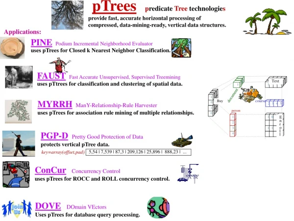
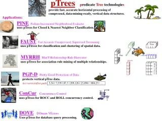
pTreespredicateTreetechnologies provide fast, accurate horizontal processing of compressed, data-mining-ready, vertical data structures. • 1 • 1 • 1 • 1 • 1 • 1 • 1 • 1 1 • 1 • 0 • 0 course 2 3 4 5 PINEPodium Incremental Neighborhood Evaluator uses pTrees for Closed k Nearest Neighbor Classification. 1 0 • 13 Text • 12 1 1 1 • 1 document • 1 1 • 1 • 1 0 Buy • 1 • 1 1 • 1 • 1 person 0 1 Enroll FAUSTFast Accurate Unsupervised, Supervised Treemining uses pTtrees for classification and clustering of spatial data. 2 3 4 MYRRHManY-Relationship-Rule Harvester uses pTrees for association rule mining of multiple relationships. PGP-DPretty Good Protection of Data protects vertical pTree data. key=array(offset,pad) 5,54 | 7,539 | 87,3 | 209,126 | 25,896 | 888,23 | ... ConCurConcurrency Control uses pTrees for ROCC and ROLL concurrency control. DOVEDOmain VEctors Uses pTrees for database query processing. Applications:
Satlog(landsat) dataset with R_G_IR1_IR2_Class. I took the 1st 1000 rows of tst as training and the 2nd 1000 rows as test. Here is the end of test: 71 79 109 92 1 0 0 0 0 84 111 128 100 1 0 0 0 0 63 87 100 87 1 0 0 0 0 59 75 96 87 1 0 0 0 0 59 75 96 75 5 0 0 0 0 63 79 93 75 5 0 0 0 0 63 68 109 92 5 0 0 0 0 R G IR1 IR2 Cs TP FP FN @IF(IR2>108 #AND# G<51 #AND# R<53, 1, 0) 13 0 2 Here are the sorted means and gaps of training: 48.54 2 58.71 5 10.17 68.77 7 10.06 75.14 1 6.37 77.34 4 2.20 89.00 3 11.66 38.60 2 58.08 5 19.48 76.83 7 18.75 90.66 4 13.83 107.62 3 16.96 112.00 1 4.38 74.76 5 80.82 7 6.07 95.43 4 14.60 112.00 3 16.57 114.68 2 2.69 120.00 1 5.32 61.22 5 63.06 7 1.84 74.85 4 11.80 88.33 3 13.47 96.86 1 8.53 119.35 2 22.49
MYRRH F A hop is a relationship, R (which hops from one entity, E, to another, F). Strong Rule Mining (SRM) finds all frequent and confidentrules, AC (Non-transitive if A,CE (the ARM case). Transitiveif AE, CF) 0 1 0 0 4 0 0 0 1 3 ct(&eACRe)mnsp) Frequency can lower bound the antecedent, consequent or both (ARM = both: Its justification is the elimination of insignificant cases. Its purpose is the tractability of SRM. 0 0 1 0 2 0 0 0 1 1 R(E,F) E 2 3 4 5 Confidence lower bds the frequency of both over the frequency of the antecedent, ct(&eARe&eCRe)/ct(&eARe)mncf The crux of SRM is frequency counts. To compare these counts meaningfully they must be on the same entity (focus entity). SRMs are categorized by the number of hops, k, whether transitive or non-transitive and by the focus entity. ARM is1-hop, E-non-transitive (A,CE) and F-focused SRM (1nF) (How does one define non-transitive in for multi-hop SRM?) 1-hop, transitive (AE,CF), F-focused SRM (1tF) APRIORI: ct(&eARe) mnsp ct(&eARe &PC) / ct(&eARe) mncf 1. (antecedent downward closure) If A is frequent, all of its subsets are frequent. Or, if A is infrequent, then so are all of its supersets. Since frequency involves only A, we can mine for all qualifying antecedents efficiently using downward closure. 2. (consequent upward closure) If AC is non-confident, then so is AD for all subsets, D, of C. So frequent antecedent, A, use upward closure to mine for all of its' confident consequents. The theorem we demonstrate throughout this section is: For transitive (a+c)-hop Apriori strong rule mining with a focus entity which is a hops from the antecedent and c hops from the consequent, if a/c is odd/even then one can use downward/upward closure on that step in the mining of strong (frequent and confident) rules. In this case A is 1-hop from F (odd, use downward closure). C is 0-hops from F (even, use upward closure). We will be checking more examples to see if the Odddownward Evenupward theorem seems to hold. 1-hop, transitive, E-focused rule, AC SRM (1tE) ct(PA&fCRf) / ct(PA) mncf |A|=ct(PA) mnsp 1. (antecedent upward closure) If A is infrequent, then so are all of its subsets. 2. (consequent downward closure) If AC is non-confident, then so is AD for all supersets, D, of C. In this case A is 0-hops from E (even, use upward closure). C is 1-hop from E (odd, use downward closure).
C G 2 3 4 5 Standard ARM can be viewed as 2tF where E=G, AC empty and S=Rtr. Thus, we have no non-transitive situation anymore, so we can drop the t verses n and call this 2F ct(&f&eAReSf & PC) / &f&eAReSf mncf 1 1 1 0 0 1 1 0 0 0 1 0 1 0 1 0 ct(PA&f&gCSgRf ) / ct(PA) mncf 2-hop transitive F-focused(focus on middle entity, F) S(F,G) AC strong if: 4 3 ct(&eARe) mnsp ct(&eARe &gCSg) / ct(&eARe) mncf 2tF 2 1 1. (antecedent downward closure) If A is infrequent, then so are all of its supersets. F 2. (consequent downward closure) If AC is non-confident, so is AD for all supersets, D. 0 1 0 0 4 0 0 0 1 3 0 0 1 0 2 3. Apriori for 2-hops: Find all freq antecedents, A, using downward closure. For each: find C1G, the set of g's s.t. A{g} is confident. Find C2G, the set of C1G pairs that are confident consequents for antecedent, A. Find C3G, the set of triples (from C2G) s.t. all subpairs are in C2G (ala Apriori), etc. 0 0 0 1 1 R(E,F) A E The number of hops from the focus are 1 and 1, both odd so both have downward closure. ct(&f&eAReSf)mnsp 2G The number of hops from the focus are 2 and 0, both even so both have upward closure. 1. (antecedent upward closure) If A is infrequent, then so for are all subsets. 2. (consequent upward closure) If AC is non-confident, so is AD for all subsets, D. ct(PA)mnsp 2E The number of hops from the focus are 0 and 2, both even so both have upward closure. 1. (antecedent upward closure) If A is infrequent, then so for are all subsets. 2. (consequent upward closure) If AC is non-confident, so is AD for all subsets, D.
3-hop ct(&eARe ct(&eARe &g&hCThSg) mnsp /ct(&eARe 3F mncf antecedent downward closure: A infreq. implies supersets infreq. A 1-hop from F (down consequent upward closure: AC noncnf implies AD noncnf. DC. C 2-hops (up 2 2 3 3 4 4 5 5 ct(&f&eAReSf) ct(&f&eAReSf &hCTh) /ct(&f&eAReSf) mnsp mncf 3G antecedent upward closure: A infreq. implies all subsets infreq. A 2-hop from G (up) consequent downward closure: AC noncnf impl AD noncnf. DC. C 1-hops (down) 1 0 1 1 0 1 0 1 0 0 0 1 0 0 1 1 ct(&eARe &glist&hCThSg ) ct(&flist&eAReSf &hCTh) / ct(&flist&eAReSf) /ct(&eARe / ct(1101 & 0011 ) / ct(&f=2,5Sf ct(&f=2,5Sf ct(1101 & 0011 & &1101 ) &1101 ) Focus on F Are they different? Yes, because the confidences can be different numbers. Focus on G. / ct(0001) = 1/1 =1 ct(0001 ) ct( 1001 &g=1,3,4 Sg ) /ct(1001) ct(PA) mnsup C H ct( 1001 &1001&1000&1100) / 2 / ct(PA) mncnf ct(PA & Rf) G S(F,G) 3E f&g&hCThSg ct( 1000 ) / 2 = 1/2 0 1 0 1 4 0 0 0 1 3 1 0 1 0 antecedent upward closure: A infreq. implies subsets infreq. A 0-hops from E (up) 2 0 0 0 1 1 consequent downward closure: AC noncnf implies AD noncnf. DC. C 3-hops (down) T(G,H) F ct(& Tg & PC) g&f&eAReSf mncnf mnsp 3H 0 1 0 0 4 0 0 0 1 3 ct(& Tg) /ct(& Tg) g&f&eAReSf g&f&eAReSf 0 0 1 0 2 antecedent downward closure: A infreq. implies all subsets infreq. A 3-hops from G (down) 0 0 0 1 1 consequent upward closure: AC noncnf impl AD noncnf. DC. C 0-hops (up) A R(E,F) E Collapse T: TC≡ {gG|T(g,h) hC} That's just 2-hop case w TCG replacing C. ( can be replaced by or any other quantifier. The choice of quantifier should match that intended for C.). Collapse T and S: STC≡{fF |S(f,g) gTC} Then it's 1-hop w STC replacing C.
4-hop 4 U(H,I) 3 2 1 C I H ct(&f&eAReSf) mnsp G S(F,G) 4G 0 1 0 1 4 0 0 0 1 3 ct(&f&eAReSf &h&iCUiTh) / ct(&f&eAReSf) 1 0 1 0 ct(&f&eAReSf &h&iCUiTh) /ct(&f&eAReSf) 2 mncf mncnf 0 0 0 1 1 T(G,H) 2 2 2 2 3 3 3 3 4 4 4 4 5 5 5 5 ct(&f&eAReSf) F mnsup G U(G,I) C Sn(G,G) I 0 1 0 0 F=G=H=genes and S,T=gene-gene intereactions. More than 3, S1, ..., Sn? ... 4 4 0 0 0 1 3 3 S1(G,G) 0 0 1 0 2 2 0 0 0 1 1 1 A (ct(S1(&eARe ct(Sn(&eARe &iCUi))+ &iCUi)) ) R(E,F) E 1 0 1 1 1 1 1 1 1 0 1 1 0 1 1 1 1 0 1 1 0 0 1 1 1 1 0 1 1 0 1 0 1 0 1 0 1 1 0 0 0 1 1 1 1 0 1 1 0 0 1 0 0 1 0 0 1 0 0 0 0 0 1 1 1 0 0 0 0 0 0 0 0 0 1 0 1 0 0 0 0 0 1 0 1 0 0 1 0 0 0 1 0 1 1 1 0 1 0 1 1 0 1 0 0 1 0 0 0 1 1 1 ct(S2(&eARe &iCUi))+... G / ( (ct(&eARe))n *ct(&iCUi) ) mncnf 0 1 0 0 4 0 0 0 1 3 If the S cube can be implemented so counts can be can be made of the 3-rectangle in blue directly, calculation of confidence would be fast. 0 0 1 1 2 0 0 1 1 1 A R(E,G) E 4G APRIORI: 1. (antecedent upward closure) If A is infrequent, then so are all of its subsets (the "list" will be larger, so the AND over the list will produce fewer ones) Frequency involves only A, so mine all qualifying antecedents using upward closure. 2. (consequent upward closure) If AC is non-confident, then so is AD for all subsets, D, of C (the "list" will be larger, so the AND over the list will produce fewer ones) So frequent antecedent, A, use upward closure to mine out all confident consequents, C. Collapse U,R: Replace C by UC; A by RA as above (not different from 2 hop? Collapse R: (RA for A, use 3-hop) Collapse U: (UC for C, use 3-hop).
5-hop C J 0 1 0 1 4 U(H,I) 0 0 0 1 3 1 0 1 0 2 0 0 0 1 1 V(I,J) I H G S(F,G) 2 2 2 3 3 3 4 4 4 5 5 5 0 1 0 1 4 0 0 0 1 3 1 0 1 0 2 ct(&f&eAReSf) 0 0 0 1 1 mnsup T(G,H) F 1 1 1 0 1 1 0 1 1 0 1 1 1 0 0 0 0 0 0 1 0 0 0 0 1 0 0 0 1 1 0 1 0 1 0 0 4 0 0 0 1 3 0 0 1 0 2 0 0 0 1 1 A R(E,F) E 5G ct( &f&eAReSf &h(&)UiTh ) / ct(&f&eAReSf) mncnf i(&jCVj) 5G APRIORI: 1. (antecedent upward closure) If A is infrequent, then so are all of its subsets (the "list" will be larger, so the AND over the list will produce fewer ones) Frequency involves only A, so mine all qualifying antecedents using upward closure. 2. (consequent downward closure) If AC is non-confident, then so is AD for all supersets, D, of C. So frequent antecedent, A, use downward closure to mine out all confident consequents, C.
6-hop C J I 0 1 0 1 4 U(H,I) 0 0 0 1 3 1 0 1 0 2 0 0 0 1 1 V(I,J) H G S(F,G) 0 1 0 1 4 0 0 0 1 3 1 0 1 0 2 0 0 0 1 1 2 2 2 2 3 3 3 3 4 4 4 4 5 5 5 5 T(G,H) F Q(D,E) E 0 1 0 0 4 0 0 0 1 3 0 0 1 0 2 0 0 0 1 1 1 1 0 1 0 1 1 1 1 0 1 1 0 1 1 1 0 1 1 0 1 1 0 0 0 1 0 0 0 0 0 0 0 0 0 0 1 1 1 0 0 1 1 0 1 0 1 0 R(E,F) A D The conclusion we have demonstrated (but not proven) is: for (a+c)-hop transitive Apriori ARM with focus the entity which is a hops from the antecedent and c hops from the consequent, if a/c is odd/even use downward/upward closure on that step in the mining of strong (frequent and confident) rules. ct( &f(& )ReSf) mnsup 6G e(&dDQd) &f(&)ReSf ct( &h(&)UiTh) / e(&dDQd) i(&jCVj) &f(& )ReSf ) ct( mncnf e(&dDQd) 6G APRIORI: 1. (antecedent downward closure) If A is infrequent, then so are all of its supersetsbsets. Frequency involves only A, so mine all qualifying antecedents using downward closure. 2. (consequent downward closure) If AC is non-confident, then so is AD for all supersets, D, of C. So frequent antecedent, A, use downward closure to mine out all confident consequents, C.
Given any 1-hop labeled relationship (e.g., cells have values from {1,2,…,n} then there is: D C M 0 1 0 1 4 R5(C,M) 0 0 0 1 3 1 0 1 0 2 0 0 0 1 1 R0(M,C) C M R3(C,M) 0 1 0 1 4 0 0 0 1 3 1 0 1 0 2 0 0 0 1 1 2 2 2 2 2 3 3 3 3 3 4 4 4 4 4 5 5 5 5 5 R4(M,C) D C F R1(C,M) M 0 1 0 0 4 0 0 0 1 3 0 0 1 0 2 0 0 0 1 1 0 0 0 0 0 1 1 1 1 1 0 0 0 0 0 0 0 0 0 0 4 1 1 1 0 1 1 0 1 1 0 1 1 0 1 1 0 0 1 0 1 1 0 1 1 0 0 0 0 0 0 0 0 0 0 1 0 1 0 0 1 1 0 0 1 1 1 0 1 R0(E,F) 0 0 0 0 0 0 0 0 0 0 0 0 0 0 0 1 1 1 1 1 3 R2(M,C) ... 0 0 0 0 0 0 0 0 0 0 1 1 1 1 1 0 0 0 0 0 2 A C 0 0 0 0 0 0 0 0 0 0 0 0 0 0 0 1 1 1 1 1 1 Rn-2(E,F) A E Rn-1(E,F) 1. a natural n-hop transitive relationship, AD, by alternating entities for each individual label value bitmap relationships. 2. cards for each entity consisting of the bitslices of cell values. E.g., netflix, Rating(Customer,Movie) has label set {0,1,2,3,4,5}, so in 1. it generates a bonafide 6-hop transitive relationship. Below, as in 2., Rn-i can be bitslices R1(A)= "Movies rated 1 by all customers in A. R2(R1(A))= "Cust who rate as 2, all R1(A) movies" = "Cust who rate as 2, all movies rated as 1 by all A-cust". R3(R2(R1(A)))= "Movies rated as 3 by all R2(R1(A)) customers" = "Movies rated as 3 by all customers who rate as 2 all movies rated as 1 by all A-customers". R4(R3(R2(R1(A))))= "Customers who rate as 4 all R3(R2(R1(A))) movies" = "Customers who rate as 4 movies rated as 3 by all customers who rate as 2 all movies rated as 1 by all A-customers". R5(R4(R3(R2(R1(A)))))= "Movies rated as 5 by all R4(R3(R2(R1(A)))) customers" = "Movies rated 5 by all customers who rate as 4 movies rated as 3 by all customers who rate as 2 all movies rated as 1 by all A-customers". R0(R5(R4(R3(R2(R1(A))))))= "Customers who rate as 0 all R5(R4(R3(R2(R1(A))))) movies" = "Cust who rate as 0 all movies rated 5 by all cust who rate as 4 movies rated as 3 by all cust who rate as 2 all movies rated as 1 by all A-cust". R0(R5(R4(R3(R2(R1(A)))))) D E.g., equity trading on a given day, QuantityBought(Cust,Stock) w labels {0,1,2,3,4,5} (where n means n thousand shares) so that generates a bonafide 6-hop transitive relationship: E.g., equity trading - moved similarly, (define moved similarly on a day --> StockStock(#DaysMovedSimilarlyOfLast10) E.g., equity trading - moved similarly2, (define moved similarly to mean that stock2 moved similarly to what stock1 did the previous day.Define relationship StockStock(#DaysMovedSimilarlyOfLast10) E.g., Gene-Experiment, Label values could be "expression level". Intervalize and go! Has Strong Transitive Rule Mining (STRM) been done? Are their downward and upward closure theorems already for it? Is it useful? That is, are there good examples of use: stocks, gene-experiment, MBR, Netflix predictor,...
Buys(C,T) =1 iff tD s.t. B(c,t)=1, B(c,t)=1 means it s.t. BB(I,c)=1 Let Types be an entity which clusters Items (moves Items up the semantic hierarchy), E.g., in a store, Types might include; dairy, hardware, household, canned, snacks, baking, meats, produce, bakery, automotive, electronics, toddler, boys, girls, women, men, pharmacy, garden, toys, farm). Let A be an ItemSet wholly of one Type, TA, and l et D by a TypesSet which does not include TA. Then: D Types (of Items) 4 3 2 1 Customers A Items 0 1 0 0 20 0 0 0 1 19 0 0 1 0 18 0 0 0 1 17 2 3 4 5 0 0 0 0 0 0 0 0 0 0 0 0 0 0 0 0 0 0 0 0 0 0 0 0 0 0 0 0 0 0 0 0 0 0 0 0 0 0 0 0 0 0 0 0 0 0 0 0 1 1 1 1 1 1 1 1 1 1 1 1 1 1 1 1 16 15 14 13 12 11 10 1 1 0 1 0 0 1 1 0 1 0 0 1 1 0 0 9 8 7 6 5 4 ct(&iABBi &tDBt) mnsp, etc. 3 2 1 BoughtBy(I,C,) AD might mean If iA s.t. BB(i,c) then tD, B(c,t) AD might mean If iA s.t. BB(i,c) then tD, B(c,t) AD might mean If iA s.t. BB(i,c) then tD, B(c,t) AD might mean If iA s.t. BB(i,c) then tD, B(c,t) AD confident might mean ct(&iABBi &tDBt) / ct(&iABBi) mncf ct(&iABBi | tDBt) / ct(&iABBi) mncf ct( | iABBi | tDBt) / ct( | iABBi) mncf AD frequent might mean ct( | iABBi &tDBt) / ct( | iABBi) mncf ct(&iABBi) mnsp ct( | iABBi) mnsp ct(&tDBt) mnsp ct( | tDBt) mnsp
A thought on impure pTrees (i.e., with predicate, 50%ones). The training set was ordered by class (all setosa's came first, then all versicolor then all virginica) so that level_1 pTrees could be chosen not to span classes much. Take an images as another example. If the classes are RedCars, GreenCars, BlueCars, ParkingLot, Grass, Trees, etc., and if Peano ordering is used, what if a class spans Peano squares completely? We now create pTrees from many different predicates. Should we created pTreeSets for many different orderings as well? This would be a one time expense. It would consume much more space, but space is not an issue. With more pTrees, our PGP-D protection scheme would automatically be more secure. So move the first column values to the far right for the 1st additional Peano pTreeSet: Move the 1st 2 columns to the right for 2nd Peano pTreeSet, 1st 3 for 3rd Peano pTreeSet..
Move the last column to the left for the 4th, the last 2 left for the 5th, the last 3 left for the 6th additional Peano pTreeSet. For each of these 6 additional Peano pTreeSets, make the same moves vertically (64 Peano pTreeSets in all), e.g., the 25th would be (starting with the 4th horizontal, directly above). For each of these 6
What about this? Looking at the vertical expansions of the 2nd additional pTreeSet (the 13th and 14th additional pTreeSets, respectively?) If we're given only pixel reflectance values for GreenCar, then we have to rely on individual pixel reflectances, right? In that case, we might as well just analyze each pixel for GreenCar characteristics. And then we would not benefit from this idea except that we might be able to data mine GreenCars using level_2 only?? Question: How are the training set classes given to us in Aurora, etc.? My question is, are we just given a set of pixels that we're told are GreenCar pixels? Or are we given anything that would allow us to use shapes of GreenCars to identify em? That is, are we given a traning set of GreenCar pixels together with their relative positions to one another - or anything like that? The green car is now centered in a level_2 pixel, assuming the level_2 stride is 16 (and the level_1 stride is 4).
Notice that the left move 3 is the same as right move 1 (and left 2 is the same as right 2; left 1 is the same as right 3.) Thus, we have only 42 = 16 orderings (not 64) at level-2; 41 = 4 at level-1; 4n at level-n. Essentially the upper right corner can be in any one of the cells in a level-n pixel and there are 4n such cells. If we always create pure1, pure0 (for complements of pure1) and GTE50% predicate trees, there would be 3*4n separate PTreeSets. Then the question is how to order pixels in a left (or up) shift? We could actually shift and then use the usual Peano? Or we could keep each cell ordering as much the same as possible (see below). One thought is to do the shifting at level-0, and percolate it upward. But we have to understand what that means. We certainly wouldn't store shifted level-0 PTreeSets since they are the same pixelization. So: construct shifted level-n pixelizations (n>0) concurrently by considering, one at a time, all level-0 pixel shifts (creating an additional PTreeSet only when it is a new pixelization (e.g., only the first level-0 pixel shift produces a new pixelization at level-1; only the first 3 at level-2, only the first 7 at level-3, etc. Throw away the bogus level-n pixels (e.g., at right throw away right column of level-2 pixels since it isn't bonefide image). Start with a fresh Z-ordering (2nd option).
RoloDex Model: 2 Entitiesmany relationships 16 DataCube Model for 3 entities, items, people and terms. 6 itemset itemset card 5 Item 4 3 2 1 Author People 2 1 2 1 2 2 3 3 4 3 3 4 4 4 5 5 5 6 7 ItemSet ItemSet antecedent Customer 1 1 1 1 1 1 1 1 5 6 16 1 1 1 Enrollments 2 1 1 1 1 1 1 1 3 Doc 1 4 movie 2 Course 3 term G 3 0 0 0 5 0 4 0 5 0 0 0 1 0 1 2 3 4 5 6 7 Doc 0 0 3 0 0 customer rates movie card 0 2 2 0 3 4 0 0 0 0 1 0 0 1 0 0 4 0 0 5 0 t 3 2 1 1 2 3 PI PI termterm card (share stem?) Gene 4 5 3 6 4 7 Relational Model: 5 6 1 People: p1 p2 p3 p4 |0 100|A|M| |1 001|T|M| |2 010|S|F| |3 011|B|F| |4 100|C|M| Items: i1 i2 i3 i4 i5 |0 001|0 |0 11| |1 001|0 |1 01| |2 010|1 |0 10| Terms: t1 t2 t3 t4 t5 t6 |1 010|1 101|2 11| |2 001|0 000|3 11| |3 011|1 001|3 11| |4 011|3 001|0 00| Relationship: p1i1 t1 |0 0| 1 |0 1| 1 |1 0| 1 |2 0| 2 |3 0| 2 |4 1| 2 |5 1|_2 1 3 Gene Exp 0 0 0 0 1 0 0 0 1 0 0 0 0 0 0 0 0 customer rates movie as 5 card 0 0 0 0 0 0 0 0 0 0 0 0 0 0 0 1 0 2 3 4 people 1 5 items 3 2 1 4 terms 3 2 1 Conf(AB) =Supp(AB)/Supp(A) MYRRHpTree-basedManY-Relationship-Rule Harvester uses pTrees for ARM of multiple relationships. Supp(A) = CusFreq(ItemSet) cust item card termdoc card authordoc card genegene card (ppi) docdoc People expPI card expgene card genegene card (ppi)
pre-computed BpTtreec 1-counts 2 BpTtreeb 1-cts 1 3 2 1 1 0 1 0 2 3 1 3 2 1 4 1 2 2 5 pre-comR5pTtreeb 1-cts R5pTtreeb&PpTreeb 1-counts 1 1 1 1 R5pTtreec 1-cts 0 1 0 1 1 1 1 1 0 1 1 1 0 1 0 0 0 0 1 0 0 0 1 0 0 0 1 1 1 1 0 0 P(B,C) R5(C,B) 0 1 0 0 0 0 0 1 0 0 1 0 0 0 0 1 APPENDIX: MYRRH_2e_2r(standard pARM is MYRRH_2e_1r ) e.g., Rate5(Cust,Book) or R5(C,B), Purchase(Book,Cust) or P(B,C) P(B,C) (S(E,F)) If cust, c, rates book, b as 5, then c purchase b. For bB, {c| rate5(b,c)=y}{c| purchase(c,b)=y} ct(R5pTreei & PpTreei) / ct(R5pTreei) mncnf ct(R5pTreei) / sz(R5pTreei) mnsp 4 3 C (E) Speed of AND: R5pTreeSet & PpTreeSet? (Compute each ct(R5pTreeb&PpTreeb).) Slice counts, bB, ct(R5pTreeb & PpTreeb) w AND? 2 1 B (F) 0 1 0 0 R5(C,B) (R(E,F)) 0 0 0 1 0 0 1 0 Given eE, If R(e,f), then S(e,f) ct(Re & Se)/ct(Re)mncnf, ct(Re)/sz(Re)mnsp 0 0 0 1 If eAR(e,f), then eBS(e,f) ct( &eARe &eBSe) / ct(&eARe) mncnf. ... Schema: size(C)=size(R5pTreeb)=size(BpTreeb)=4 size(B)=size(R5pTreec)=size(BpTreec)=4 If eAR(e,f), then eBS(e,f) ct( &eARe OReBSe) / ct(&eARe) mncnf. ... If eAR(e,f), then eBS(e,f) ct( OReARe &eBSe) / ct(OReARe) mncnf. ... If eAR(e,f), then eBS(e,f) ct( OReARe OReBSe) / ct(OReARe) mncnf. ... C\B1 2 3 4 2 1 0 1 1 3 0 1 0 1 4 0 1 0 0 5 1 1 0 0 Consder 2 Customer classes, Class1={C=2|3} and Class2={C=4|5}. Then P(B,C) is TrainingSet: Book=4 is very discriminative of Class1 and Class2, e.g., Class1=salary>$100K Then the DiffSup table is: B=1 B=2 B=3 B=4 0 1 1 2 P1={B=1|2} P2={B=3|4} C1 0 1 C2 1 0 DS 1 1 P1 [and P2, B=2 and B=3] is somewhat discriminative of the classes, whereas B=1 is not.. Are "Discriminative Patterns" covered by ARM? E.g., does the same information come out of strong rule mining? Does "DP" yield information across multiple relationships? E.g., determining the classes via the other relationship?
SL SW PL rnd(PW/10) 4 4 1 0 5 4 2 0 5 3 2 0 5 4 2 0 5 3 1 0 0 2 5 2 6 3 5 1 6 3 3 1 5 3 5 1 6 3 4 1 7 3 6 2 6 3 5 2 7 3 5 1 7 3 5 2 7 3 5 2 stride=10 level-1 val SL SW PL PW setosa 38 38 14 2 setosa 50 38 15 2 setosa 50 34 16 2 setosa 48 42 15 2 setosa 50 34 12 2 versicolor 1 24 45 15 versicolor 56 30 45 14 versicolor 57 28 32 14 versicolor 54 26 45 13 versicolor 57 30 42 12 virginica 73 29 58 17 virginica 64 26 51 22 virginica 72 28 49 16 virginica 74 30 48 22 virginica 67 26 50 19 Making 3-hops: Use 4 feature attributes of an entity. For IRIS(SL,SW,PL,PW). L(SL,PL), P(PL,PW), W(PW,SW) Let ASL be {6,7} and CPW be {1,2} SW=0 1 2 3 4 5 6 7 S0 0 0 0 0 0 0 0 0 0 0 0 0 0 0 0 0 0 0 0 0 0 0 0 0 0 0 0 0 0 0 0 0 1 0 0 0 0 0 0 0 0 0 0 0 0 0 0 0 0 0 0 0 0 0 0 0 0 0 0 0 0 0 0 PW 00 1 1 0 0 0 0 0 P 10 0 0 1 1 1 0 0 20 0 0 0 0 1 1 0 30 0 0 0 0 0 0 0 40 0 0 0 0 0 0 0 50 0 0 0 0 0 0 0 60 0 0 0 0 0 0 0 70 0 0 0 0 0 0 0 PL=0 1 2 3 4 5 6 7 PL=0 1 2 3 4 5 6 7 00 0 0 0 0 1 0 0 L 10 0 0 0 0 0 0 0 20 0 0 0 0 0 0 0 30 0 0 0 0 0 0 0 40 1 0 0 0 0 0 0 50 0 1 0 0 1 0 0 60 0 0 1 1 1 0 0 70 0 0 0 0 1 1 0 SL
2-hop transitive rules (specific examples) E(S,C) C 4 3 2 D 1 S A 0 1 0 0 4 0 0 0 1 3 0 0 1 0 2 2 2 2 3 3 3 4 4 4 5 5 5 0 0 0 1 1 P(B,S) B PJ(C,I) I 1 0 1 1 1 1 1 1 0 0 1 1 1 0 1 1 0 0 1 0 1 0 0 1 0 0 1 1 0 1 0 0 0 0 0 0 1 1 0 0 1 0 0 1 1 0 1 0 4 3 2 D 1 C A 0 1 0 0 4 0 0 0 1 3 0 0 1 0 2 0 0 0 1 1 PD(I,C) I B(P,I) I 4 3 2 D 1 P A 0 1 0 0 4 0 0 0 1 3 0 0 1 0 2 0 0 0 1 1 O(E,P) E AD: If bAP(b,s), then cDE(s,c) is a strong rule if: ct(&bAPb) minsupp ct(&bAPb &cDEc) / ct(&bAPb) minconf 2-hop Enroll Book If a student Purchases every book in A, then that student is likely to enroll in every course in D, and lots of students purchase every book in A. In short, P(A,s) E(s,D) is confident and P(A,s) is frequent 2-hop Purchase Dec/Jan AD: If iAPD(i,c), then iDPJ(c,i) is a strong rule if: ct(&iAPDi) minsupp ct(&iAPDi &iDPJi) / ct(&iAPDi) minconf If a customer Purchases every item in A in December, then that customer is likely to purchase every item in D in January, and lots of customers purchase every item in A in December: PD(A,c)PJ(c,D) conf and PD(A,c) freq. 2-hop Event Buy AD: If eAO(e,p), then iDB(p,i) is a strong rule if: ct(&eAOe) minsupp ct(&eAOe &iDBi) / ct(&eAOe) minconf If every Event in A occurred in a person's life last year, then that person is likely to buy every item in D this year, and lots of people had every Event in A occur last year: O(A,p)B(p,D) conf and O(A,p) freq.
AD: If eAO(e,s), then mDT(s,m) is a strong rule if: B(P,I) T(C,M) T(S,M) M M I 4 4 4 3 3 3 2 2 2 D D D 1 1 1 P C S A A A 0 0 0 1 1 1 0 0 0 0 0 0 4 4 4 0 0 0 0 0 0 0 0 0 1 1 1 3 3 3 0 0 0 0 0 0 1 1 1 0 0 0 2 2 2 2 2 2 3 3 3 4 4 4 5 5 5 0 0 0 0 0 0 0 0 0 1 1 1 1 1 1 O(E,S) O(E,C) F(P,P) P E E 0 1 1 1 0 1 1 1 0 1 1 1 1 0 1 0 0 1 0 1 1 1 0 0 1 0 0 0 0 1 0 0 0 0 0 1 0 0 1 0 0 1 0 1 1 1 1 0 2-hop stock trading ct(&eAOe) minsupp ct(&eAOe &mDTm) / ct(&eAOe) minconf If every Event in A occurs for a company in time period 1, then the price of that stock experienced every move in D time period 2, and lots of companies had every Event in A occur in period 1: O(A,s)T(s,D) conf and O(A,s) freq.(T=True; e.g., m=1 down a lot, m=2 down a little, m=3 up a little, m=4 up a lot.) AD: If eAO(e,c), then mDT(c,m) is a strong rule if: 2-hop commodity trading ct(&eAOe) minsupp ct(&eAOe &mDTm) / ct(&eAOe) minconf If every Event in A occurs for a commodity in time period 1, then the price of that commodity experienced every move in D time period 2, and lots of commodities had every Event in A occur in period 1: O(A,c)T(c,D) conf and O(A,c) freq. AD: If pAP(p,q), then iDB(p,i) is a strong rule if: 2-hop facebook friends buying ct(&pAFp) minsupp ct(&pAFp &iDBi) / ct(&pAFp) minconf F(p,q)=1 iff q is a facebook friend of p. B(p,i)=1 iff p buys item i. People befriended by everyone in A (= &pAFp denoted FA for short ) likely buy everything in D. And FA is large. So every time a new person appears in FA that person is sent ads for items in D.
2 5 1 2 3 4 4 5 3 2 5 5 1 1 0 1 0 0 1 1 0 0 1 0 0 0 1 1 I I B(C,I) B'(IL,I) 1 1 0 4 4 3 1 0 0 3 2 0 1 1 2 1 1 1 1 0 Bil=2 = Bc=3OR Bc=5 Bil=1 = Bc=2 1 2 3 IL C A IL Bil=3 = Bc=4 5 1 1 1 4 0 1 0 I AO(A,IL) How do we construct interesting 2-hop examples? Method-1: Use a feature attribute of a 1-hop entity. Start with a 1-hop, e.g., customers buy items, stocks have prices or people befriend people then focus on one feature attribute of one of the entities. The relationship is the projection of that entity table onto the feature attribute and the entity id attribute (key) e.g. Age, Gender, Income Level, Ethnicity, Weight, Height... of people or customer entity These are not bonafide 2-hop transitive relationships since they are many-to-one relationships, not a many-to-many (because the original entity is the primary key of its feature table). Thus, we don't get a fully transitive relationship since collapsing the original entity leaves nearly the same information as the transitive situation was intended to add. Here is an example. If, from the new transitive relationship, AgeIsAgeOfCustomerPurchasedItem, Customer is collapsed we have AgePurchaseItem and the Customer-to-Age info is still available to us in the Cust table. The relationship between Customers and Items is lost, but presumably, the reason for mining, AgeIsAgeOfCustomerPurchaseItem is to find AgePurchaseItem rules independent of the Customers involved. Then when a high confidence Age implies Item rule is found, the Customers who are of that age can be looked up from the Customer feature table and sent a flyer for that item. Also, in CustomerPurchaseItem, the antecedent, A, could have been chosen to be an age-group. So most AgePurchaseItem info would come out of CustomerPurchaseItem directly. Given a 1-hop relationship, R(E,F) and a feature attribute, A of E, if there is a pertinent way to raise E up the semantic hierarchy (cluster it) producing E', then the relationship between A and E ' is many-to-many, e.g., cluster Customers by Income Level, IL. Then AgeIsAgeOfIL is a many-to-many relationship. Note, what we're really doing here is using the many-to-many relationship between two feature attributes in one of the entity tables and then replacing the entity by the second feature. E.g., if B(C,I) is a relationship, and IL is a feature attribute in the entity table C(A,G,IL,E,W,H), then clustering (Classifying) C by IL produces a relationship, B'(IL,I), given by B'(il,i)=1 iff B(c,i)=1 for 50% of cil, which is many-to-many provided IL is not a candidate key. So from the 1-hop relationship, CB(C,I)I, we get a bonafide 2-hop relationship, AAO(A,IL)ILB'(IL,I)I. ct(&aAAOe)mnsp ct(&aAAOa&gCB'g)/ct(&aAAOa)mncf ct( AOa=4)mnsp ct(AOa=4 &g=3,4B'g )/ct(AOa=4 )mncf C ct( 010)mnsp ct(010 &100&110)/ ct(010) mncf 1 mnsp 0 / 1 mncf ct(&cC(A)Bc)mnsp ct(&cC(A)Bc &IC)/ct(&cC(A)Bc)mncf ct( Bc=3 )mnsp ct(Bc=3 &0011)/ct(Bc=3 )mncf A ct( 0101)mnsp ct(0101&0011)/ct(0101)mncf So these are different rules. 2 mnsp 1 / 2 mncf
SL SW PL rnd(PW/10) 4 4 1 0 5 4 2 0 5 3 2 0 5 4 2 0 5 3 1 0 0 2 5 2 6 3 5 1 6 3 3 1 5 3 5 1 6 3 4 1 7 3 6 2 6 3 5 2 7 3 5 1 7 3 5 2 7 3 5 2 stride=10 level-1 val SL SW PL PW setosa 38 38 14 2 setosa 50 38 15 2 setosa 50 34 16 2 setosa 48 42 15 2 setosa 50 34 12 2 versicolor 1 24 45 15 versicolor 56 30 45 14 versicolor 57 28 32 14 versicolor 54 26 45 13 versicolor 57 30 42 12 virginica 73 29 58 17 virginica 64 26 51 22 virginica 72 28 49 16 virginica 74 30 48 22 virginica 67 26 50 19 Method-2: Use 3 feature attribute of an entity.Start with an Entity (e.g., IRIS(SL,SW,PL,PW). Take 3 attributes SL,PL,PW; form 2 many-to-many relationships L(SL,PL) and P(PL,PW) in which a cell value is 1 iff there is a IRIS sample with those values (Could also cluster IRIS on SW first then add PL and PW, so that the key, IRIS-ID is involved.) Let ASL be {6,7} and CPW be {1,2} ct(&aALa) mnsp ct(&aALa&cCPc)/ct(&aALa) mncf ct(00000100)mnsp ct(0000 0100& 0000 0100)/ct(0000 0100)mncf 1 mnsp 1 / 1 mncf PW=00 1 1 0 0 0 0 0 10 0 0 1 1 1 0 0 20 0 0 0 0 1 1 0 30 0 0 0 0 0 0 0 40 0 0 0 0 0 0 0 50 0 0 0 0 0 0 0 60 0 0 0 0 0 0 0 70 0 0 0 0 0 0 0 PL=0 1 2 3 4 5 6 7 So, with very high confidence, SL[55,74] PL PW[5,24], however the support of this rule is very low. What about the 1-hop version? (aA)(SLPWaC) sup conf=ct(ORaASLPWa&pTreeC) / ct(ORaASLPWa) PW=0 12 3 4 5 6 7 SL=00 0 1 0 0 0 0 0 10 0 0 0 0 0 0 0 20 0 0 0 0 0 0 0 30 0 0 0 0 0 0 0 41 0 0 0 0 0 0 0 51 1 0 0 0 0 0 0 60 1 1 0 0 0 0 0 70 1 1 0 0 0 0 0 conf=ct( 0110 0000& 0110 0000) / ct( 0110 0000) conf= 2/2 = 1 Supp=2 PL=0 1 2 3 4 5 6 7 SL=00 0 0 0 0 1 0 0 10 0 0 0 0 0 0 0 20 0 0 0 0 0 0 0 30 0 0 0 0 0 0 0 40 1 0 0 0 0 0 0 50 0 1 0 0 1 0 0 60 0 0 1 1 1 0 0 70 0 0 0 0 1 1 0 What's the difference? The 1-hop says "if SLA then PW will likely C. 2-hop says "If all SL in A are related to a PL then that PL is likely to be related to all PW in C." These are different. 2-hop seems convoluted. Why? 2-hops from one table may always make less sense than the corresponding direct 1-hop. How do you mine out all confident (or all strong) rules?