Download
1 / 47
670 likes | 1.16k Vues
Energy-Dispersive X-ray Spectrometry in the AEM. Charles Lyman. Based on presentations developed for Lehigh University semester courses and for the Lehigh Microscopy School. Why Do EDS X-ray Analysis in TEM/STEM?. Spatial resolution 2-20 nm (10 3 times better than SEM/EPMA)

E N D
Energy-Dispersive X-ray Spectrometry in the AEM Charles Lyman Based on presentations developed for Lehigh University semester courses and for the Lehigh Microscopy School
Why Do EDS X-ray Analysis in TEM/STEM? • Spatial resolution • 2-20 nm (103 times better than SEM/EPMA) • Elemental detectability • 0.1 wt% - 1 wt%, depending on the specimen (~same as SEM/EDS) • Can use typical TEM specimens (t ~ 50-500 nm) • EELS requires specimens < 20-30 nm • Straightforward microanalysis • Qualitative analysis => Which element is present? • Quantitative analysis => How much of the element is present? • Easy x-ray mapping
Example of an X-ray Spectrum 2 Types of X-rays • Characteristic x-rays • elemental identification • quantitative analysis • Continuum x-rays • background radiation • must be subtracted for quantitative analysis Example of EDS x-ray spectrum from Goldstein et al., Scanning Electron Microscopy and X-ray Microanalysis, Springer, 2003.
Continuum X-rays • Interactions of beam electrons with nuclei of specimen atoms • Accelerating electric charge emits electromagnetic radiation • Here the acceleration is a change in direction • The good • The shape of the continuum is a valuable check on correct operation • The not-so-good • I bkg increases as ib increases • I bkg is proportional to Zmean of specimen • Imax bkgrises as beam energy rises • Peak-to-background ratio • Ratio of Ichar / Ibkg sets limit on elemental detectability Continuum x-rays Absorption of continuum from Goldstein et al., Scanning Electron Microscopy and X-ray Microanalysis, Springer, 2003.
Generation of Characteristic X-rays • Mechanism • Fast beam electron has enough energy to excite all atoms in periodic table • Ionization of electron from the K-, L-, or M-shell • X-ray is a product of de-excitation • Example • Vacancy in K-shell • Vacancy filledfrom L-shell • Emission of a Ka x-ray(or a KLL Auger electron) • Important uses • Qualitativeuse x-ray energy to identify elements • Quantitativeuse integrated peak intensity to determine amounts of elements
Compute Energy of Sodium Ka Line Beam electron If beam E > EK, then a K-electron may be ionized: X-ray energy is the difference between two energy levels: L M K Energy levels EK and EL3 are in Bearden's "Tables of X-ray Wavelengths and X-ray Atomic Energy Levels" in older editions of the CRC Handbook of Chemistry and Physics For sodium (Z=11): EK = 1072 eV EL3 = 31 eV Beam electron loses EK For Na only see one peak since the Kb is only 26 eV from the Ka line
Families of Lines If K-series excited, will also have L-series Note: this is a simplified version of Goldstein Figure 6.9 showing only lines seen in EDS
Fluorescence Yield • = fraction of ionization events producing characteristic x-rays • the rest produce Auger e– • increases with Z • K typical values are: • 0.03 for carbon (12) K-series @ 0.3 keV • 0.54 for germanium (32) K-series @ 9.9 keV • 0.96 for gold (79) K-series @ 67 keV • X-ray production is inefficient for low Z lines (e.g., O, N, C) since mostly Augers produced • for each shell: KLM • X-ray production is inefficient for L-shell and M-shell ionizations since • LandM always < 0.5: L = 0.36 for Au (79) M = 0.002 for Au (79) from Goldstein et al., Scanning Electron Microscopy and X-ray Microanalysis, Springer, 2003.
X-ray Absorption and Fluorescence • X-rays can be absorbed in the specimen and in parts of the detector • Certain x-rays fluoresce x-rays of other elements • X-rays of element A can excite x-rays from element B • Energy of A photon must be close to but above absorption edge energy of element B • Example: Fe Ka (6.40 keV) can fluoresce the Cr K-series (absorption edge at 5.99 keV) Greater absorption when -- x-ray energy is just above absorber absorption edge -- path length t is large
EDS Dewar, FET, Crystal • LN dewar is most recognizable part • To cool FET and crystal • Actual detector is at end of the tube • Separated from microscope by x-ray window • Crystal and FET fitted as close to specimen as possible • Limited by geometry inside specimen chamber Schematic courtesy of Oxford Instruments
Electron-Hole Pair Creation Absorption of x-ray energy excites electrons • From filled valence band or states within energy gap Energy to create an electron-hole pair • = 3.86 eV @ 77K (value is temperature dependent) Within the intrinsic region • Li compensates for impurity holes • Ideally # electrons = # holes • # electron-hole pairs is proportional to energy of detected x-ray Conduction band Excited e- Donor Energy Energy gap Acceptor Hole Valence band For Cu Ka: 8048eV/3.8 eV = 2118 e-h pairs (after drawing by J. H. Scott)
–1000 V bias Details of Si(Li) Crystal Ice? Anti-reflective Al coating 30 nm Gold electrode Gold electrode 20 nm Silicon inactive layer (p-type) ~100 nm X-ray Electrons Holes (+) (–) Window Be, BN, diamond, polymer 0.1 mm — 7 mm Active silicon (intrinsic) 3 mm (after drawing by J. H. Scott)
X-ray Pulses to Spectrum spectrum charge staircase slow amplifier analog-to-digital converter energy bins collects e-h as charge fast amplifier from Goldstein et al., Scanning Electron Microscopy and X-ray Microanalysis, Springer, 2003.
Slow EDS Pulse Processing • EDS can process only one photon at a time • A second photon entering, while the first photon pulse is being processed, will be combined with the first photon • Photons will be recorded as the sum of their energies • X-rays entering too close in time are thrown away to prevent recording photons at incorrect energies • Time used to measure photons that are thrown away is “dead time” • Lower dead time -> fewer artifacts • Higher dead time -> more counts/sec into spectrum • Processor extends the “live time” to compensate fast amplifier slow amplifier slower amplifier Counting is linear up to 3000 cps (20-30% dead time) from Goldstein et al., Scanning Electron Microscopy and X-ray Microanalysis, Springer, 2003.
Things for Operator to Check • Detector Performance • Energy resolution (stamped on detector) • Incomplete charge collection (low energy tails) • Detector window (thin window allows low-energy x-ray detection) • Detector contamination (ice and hydrocarbon) • Count rate linearity (counts vs. beam current) • Energy calibration (usually auto routine) • Maximum throughput (set pulse processor time constant to collect the most x-rays in a given clock time with some decrease in energy resolution) Topics in red explained in next few slides
Energy Resolution • Natural line width ~2.3 eV (Mn Ka) • measured full width at half maximum (FWHM) • Peak width increases with statistical distribution of e-h pairs created and electronic noise: • Measured with 1000 cps at 5.9 keV • Mn Kaline E = x-ray energy N = electronic noise F = Fano factor (~0.1 for Si) E = 3.8 eV/electron-hole pair Mn Kaline from Williams and Carter, Transmission Electron Microscopy, Springer, 1996.
X-ray Windows • Transmission curve for a “windowless” detector • Note absorption in Si • Transmission curves for several commercially available windows • Specific windows are better for certain elements from Goldstein et al., Scanning Electron Microscopy and X-ray Microanalysis, Springer, 2003.
Ice Build Up on Detector Surface • All detectors acquire an ice layer over time • Windowless detector in UHV acquires ~ 3µm / year • Test specimens • NiO thin film (Ni La / Ni Ka) • Cr thin film (Cr La / Cr Ka) • Check L-to-K intensity ratio for Ni or Cr • L/K will decrease with time as ice builds up • Warm detector to restore (see manufacturer) Windowless detector Immediately after warmup After operating 1 year Courtesy of J.R. Michael
Spectrometer Calibration • Calibrate spectrum using two known peaks, one high E and one low E • NiO test specimen (commercial) • Ni Ka (high energy line) at 7.478 keV • Ni La (low energy line) at 0.852 keV • Cu specimen • Cu Ka (high energy line) at 8.046 keV • Cu La (low energy line) at 0.930 keV • Calibration is OK if peaks are within 10 eV of the correct value • Calibration is important for all EDS software functions 0.930 keV 8.046 keV from Goldstein et al., Scanning Electron Microscopy and X-ray Microanalysis, Springer, 2003.
Artifacts in EDS Spectra • Si "escape peaks” • Si Ka escapes the detector • Carrying 1.74 keV • Small peak ~ 1% of parent • Independent of count rate • Sum peaks • Two photons of same energy enter detector simultaneously • Count of twice the energy • Only for high count rates • Si internal fluorescence peak • Photon generated in dead layer • Detected in active region from Williams and Carter, Transmission Electron Microscopy, Springer, 1996
Escape peaks Si internal fluor. System peaks Sum peaks Expand Vertically to See EDS Artifacts from Goldstein et al., Scanning Electron Microscopy and X-ray Microanalysis, Springer, 2003.
Usually fixed by manufacturers of EDS and TEM EDS-TEM Interface • We want x-rays to come from just under the electron probe, BUT… • TEM stage area is a harsh environment • Spurious x-rays, generated from high energy x-rays originating from the microscope illumination system bathe entire specimen • High-energy electrons scattered by specimen generate x-rays • Characteristic and continuum x-rays generated by the beam electrons can reach all parts of stage area causing fluorescence • Detector can't tell if an x-ray came from analysis region or from elsewhere
The Physical Setup • Want large collection angle, W • Need to collect as many counts as possible • Want large take-off angle, a • But W reduced as a is increased • Compromise by maxmizing W with a ~ 20˚ at 0˚ tilt angle • can always increase a by tilting specimen toward detector -- but this increases specimen interaction with continuum from specimen from Williams and Carter, Transmission Electron Microscopy, Springer, 1996
Orientation of Detector to Specimen • Detector should have clear view of incident beam hitting specimen • specimen tilting eucentric • specimen at 0˚ tilt • Identify direction to detector within the image • Analyze side of hole "opposite the detector” • Keep detector shutter closed until ready to do analysis EDS detector Rim Edge of hole furthest from detector Thinned Detector from Williams and Carter, Transmission Electron Microscopy, Springer, 1996 Top view of disc
Spurious X-rays in the Microscope • Pre-Specimen Effects • spurious x-rays => hole count due to column x-rays and stray electrons • spurious x-rays => poor beam shape from large C2 aperture • Post-Specimen Scatter • system x-rays => elements in specimen stage, cold finger, apertures, etc. • spurious x-rays => excited by electrons and x-rays generated in specimen • Coherent Bremsstrahlung • extra peaks from specimen effects on beam-generated continuous radiation The analyst must understand these effects to achieve acceptable qualitative and quantitative results
Test for Spurious X-rays Generated in TEM • Detector for x-rays from illumination system • thick, high-Z metal acts as “hard x-ray sensor" • Uniform NiO thin film used to normalize the spurious "in hole" counts, thus • NiO film on Mo grid* Electron beam Beam-generated Ni K x-ray (good) Spurious (bad) Mo K-series NiO film on C Hole Mo grid bar - “on film” results ~ “in hole” results - Usually take inverse “hole count” ratio Hard x-ray from illumination system * see Egerton and Cheng, Ultramicroscopy 55 (1994) 43-54
Spectrum from NiO/Mo Measure in center of grid square on NiO/Mo specimen • Spurious x-rays • Inverse hole count (Ni Ka/ Mo Ka) • Want high inverse hole count • Fiori P/B ratio • Ni Ka/B(10 eV) • Increases with kV • Want high to improve element detectability Maximize P/B ratio for Ni Ka Minimize spurious Mo x-rays by using thick C2 aperture Egerton and Cheng, Ultramicroscopy 55 (1994) 43-54
Better Less good Figures of Merit for an AEM • Fiori PBR = full width of Ni Ka divided by 10 eV of background • (Ni Ka) / ( Mo Ka) is inverse hole count Obviously, we want to use the highest kV from Williams and Carter, Transmission Electron Microscopy, Springer, 1996
Beam Shape and X-ray Analysis • Calculated probes (from Mory, 1985) • Effect on x-ray maps (from Michael, 1990) C2 aperture too large correct C2 aperture size “witch’s hat” beam tail excites x-rays Properly limited Spherically aberrated
Qualitative Analysis Which elements are present? • Collect as many x-ray counts as possible • Use large beam current regardless of poor spatial resolution with large beam • Analyze thicker foil region, except if light elements x-rays might be absorbed • Scan over large area of single phase => avoid spot mode • Use more than one peak to confirm each element
Qualitative Analysis Setup 1 Specimen • Use thin foils, flakes, or films rather than self-supporting disks to reduce spurious x-rays (not always possible) • Orient specimen so that EDS detector is on the side of the specimen hole opposite where you take your analysis • Collect x-rays from a large area of a single phase • Choose thicker area of specimen to collect more counts • Tilt away from strong diffracting conditions • (no strong bend contours) • Operate as close to 0˚ tilt as possible (say, 5˚ tilt toward det.)
Qualitative Analysis Setup 2 Microscope Column • Use highest kV of microscope • Use clean, top-hat Pt aperture in C2 to minimize “hole count” effect • Minimize beam tails • (C2 aperture or VOA should properly limit beam angle) • Use ~ 1 nA probe current to maximize count rate • This may enlarge the electron beam (analyze smaller regions later) • Remove the objective aperture
Qualitative Analysis Setup 3 X-ray Spectrometer • Ensure that detector is cranked into position • Keep detector shutter closed until you are ready to analyze • Use widest energy range available (0-20 keV is normal) • 0–40 keV for Si(Li) detector • 0–80 keV for intrinsic Ge detector • Choose short detector time constant (for maximum countrate) • Count for a long time – 100-500 live sec
Peak Identification • Start with a large, well-separated, high-energy peak • Try the K-family • Try the L-family • Try the M-family • Remember -- these families are related • Check for EDS artifacts • Repeat for the next largest peak • Important: • Use more than one peak for identification • If peak too small to "see", collect more counts or forget about identifying that peak; peak should be greater than 3B1/2
M-series L-series K-series Chart of X-ray Energies (0-20 keV) from Goldstein et al., Scanning Electron Microscopy and X-ray Microanalysis, Springer, 2003
Chart of X-ray Energies (0-5 keV) from Goldstein et al., Scanning Electron Microscopy and X-ray Microanalysis, Springer, 2003 M-series L-series K-series
Some Peaks will Look Similar • At low energies each series collapses to a single line • From 1 keV to 3 keV, the K, L, or M lines all look similar • At 2.0 keV: • Z = 15 (P) Ka @ 2.013 keV • Z = 40 (Zr) La @ 2.042 • Z = 77 (Ir) Ma @ 1.977 M-series Z L-series K-series after Goldstein et al., Scanning Electron Microscopy and X-ray Microanalysis, Springer, 2003
Unknown #1 Energy (keV)
Data Analysis for Unknown #1 26 6.4 Fe(26) Ka 4.5 7.0 Fe(26) Kb 4.9
Unknown #1 from xray.optics.rochester.edu/.../spr04/pavel/
Unknown #2 after www.pentrace.com/ nib030601003.html
Analysis of Unknown #2 Start
W Ma Elements present major: W, Ru trace: Fe, Cu, C W La Ru La W Ll W Mz Fe Ka,b W Lb1,2 W Lg1,3 C Cu Qualitative Analysis
Automatic Qualitative Analysis? Check the results of every automatic qualitative analysis • Are suggested elements reasonable?Tc and Pm are unusual, Cl and S are not 2. Do not use peak energy alone to identify • Lines of other elements may have the same energy • Consider logic of x-ray excitation • All lines of an element are excited in TEM/STEM (100-300 kV) • If L-series indicated, K-series must be present • If M-series indicated, L-series must be present
Automatic Qualitative Analysis Blunders Identification by peak energy alone without considering x-ray families or peak shape Identification without considering other lines of same element from Newbury, Microsc. Microanal. 11 (2005) 545-561
Summary • EDS in the TEM has more pitfalls than in SEM • Use the highest kV available • Understand the effects of: • detector-specimen geometry • spurious x-rays from the illumination system • post-specimen scatter • beam shape and spatial resolution => the “witch’s hat” • Identify every peak in the spectrum • Even artifact peaks • Forget peaks of intensity < 3 x (background)1/2 • Collect as many counts as possible • Use large enough beam size to obtain about 1 nA current • Qualitative analysis use: • use long counting times or • thicker electron-transparent regions with a short pulse processor time constant, if appropriate • Assume data might be used for later quantitative analysis (determine t if possible)