US Executions 1984-2005: Scatter Plot Analysis
Analyze the number of executions in the US from 1984 to 2005 using a scatter plot. Follow steps to align and enter data in lists, set window values, and create a visual representation. Utilize STAT PLOT for formatting and interpretation.

US Executions 1984-2005: Scatter Plot Analysis
E N D
Presentation Transcript
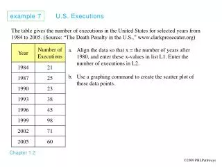
example 7 U.S. Executions Chapter 1.2 The table gives the number of executions in the United States for selected years from 1984 to 2005. (Source: “The Death Penalty in the U.S.,” www.clarkprosecuter.org) Align the data so that x = the number of years after 1980, and enter these x-values in list L1. Enter the number of executions in L2. Use a graphing command to create the scatter plot of these data points. 2009 PBLPathways
The table gives the number of executions in the United States for selected years from 1984 to 2005. (Source: “The Death Penalty in the U.S.,” www.clarkprosecuter.org) Align the data so that x = the number of years after 1980, and enter these x-values in list L1. Enter the number of executions in L2.
The table gives the number of executions in the United States for selected years from 1984 to 2005. (Source: “The Death Penalty in the U.S.,” www.clarkprosecuter.org) Align the data so that x = the number of years after 1980, and enter these x-values in list L1. Enter the number of executions in L2. Use a graphing command to create the scatter plot of these data points.
The table gives the number of executions in the United States for selected years from 1984 to 2005. (Source: “The Death Penalty in the U.S.,” www.clarkprosecuter.org) Align the data so that x = the number of years after 1980, and enter these x-values in list L1. Enter the number of executions in L2. Use a graphing command to create the scatter plot of these data points.
The table gives the number of executions in the United States for selected years from 1984 to 2005. (Source: “The Death Penalty in the U.S.,” www.clarkprosecuter.org) Use a graphing command to create the scatter plot of these data points. x
The table gives the number of executions in the United States for selected years from 1984 to 2005. (Source: “The Death Penalty in the U.S.,” www.clarkprosecuter.org) Use a graphing command to create the scatter plot of these data points. x
The table gives the number of executions in the United States for selected years from 1984 to 2005. (Source: “The Death Penalty in the U.S.,” www.clarkprosecuter.org) Use a graphing command to create the scatter plot of these data points. x
The table gives the number of executions in the United States for selected years from 1984 to 2005. (Source: “The Death Penalty in the U.S.,” www.clarkprosecuter.org) Use a graphing command to create the scatter plot of these data points.
Clear the lists Press the key. Since lists L1 and L2 may have data in them already, you’ll start by selecting 4: ClrList. Press . This pastes ClrList on the Home Screen. Now you need to indicate the lists you want to clear. Press followed by . You can enter as many lists as you want as long as they are separated by .
Alternate method for clearing lists You can also clear a list by pressing and selecting 1: Edit. This takes you to the list editor. Move your cursor to the top of the column that you want to clear. To clear the list, press . The entries in that column will be cleared. You can move the cursor to the tops of other columns and clear those too.
Enter the data points Press the key. Press to select 1:Edit or move the cursor to 1:Edit and press . This brings you to the screen where you can enter the data in the lists. Enter the Years from 1980-values in list L1. Use the down arrow , right arrow or to move from line to line or column to column. Enter the Number of executions-values in L2.
Set the window Press the key. After you examine the data, choose window values that include these values and some “space” above and below the highest and lowest values of x and y. Set the window elements to Xmin = 0, Xmax = 30, Xscl = 5, Ymin = 0, Ymax = 120, and Yscl = 20. Press the down arrow or to move from line to line.
Use STAT PLOT to turn on and format the scatter plot of data points • Press to access STAT PLOT. • Select 1: Plot 1 ON, press . • Select Type: first one for a scatter plot – individual points, press . • On the same screen select • XList: L1or whichever list has the x-data • YList: L2or whichever list has the y-data • Mark: any one you wish
Press the key to see the scatter plot. Use and the right arrow to move from point to point. The x and y coordinates of each point are displayed at the bottom of the screen. P1:L1,L2 is displayed in the upper left hand corner of the screen. This tells you that you are on Plot 1, the x’s are from list L1, and the y’s are from list L2. You can also turn a STAT PLOT on or off from the equation editor. To access the equation editor, press .
Use the arrow keys to navigate the cursor to Plot 1, Plot 2, or Plot 3. You can turn a plot on by highlighting the appropriate plot. Press to turn the plot on or off.