3.1
3.1. Characterization of waiting systems Notation Queuing strategies Prior i ties Behavi o ur of requests. What about these ?. Characterization 1. . Characterization of systems. Kendall notation. Traffic processes ( distributions ):. Characterization 2. .


3.1
E N D
Presentation Transcript
3.1 Characterization of waiting systems Notation Queuing strategies Priorities Behaviour of requests
What about these ? Characterization 1. Characterization of systems Kendallnotation Trafficprocesses (distributions):
Characterization 2. Complete specification: Further notations: K = n is a loss system Ab csoportos érkezés (bulk or batch arrival). Bb csoportos kiszolgálás, (bulk or batch service) C ütemezett kiszolgálás (clocked service)
Characterization 3. Queuing strategies For the three above-mentioned disciplines the total waiting time for all customers is thesame. The queueing discipline only decides how waiting time is allocated to the individualcustomers.
Characterization 4. Static disciplines, depending on arrival times or holding times Dynamic disciplines. Strategy depends on the time spent in the system
Characterization 5. Priorities The strategies mentioned may apply in each priority class
Characterization 6. Behaviourof requests (customers)
3.2 Erlang’s delay system M|M|n Detailed mathematics serve the better understanding of essential results For furtherdetails see: Textbook, Section 9.
Erlang – M/M/n 1. • The system • nuniform servers • full accessibility • ∞ waiting positions • PCT I flow of demands The state of the system is given by the numberof all (served and waiting) requests.
Erlang – M/M/n 2. A=/μ Stateequations
Erlang – M/M/n 3. Probability of waiting: a request arrives and all servers are occupied ______________________________________________________ a request arrives anytime Erlang Cformula: Designations: Probability of immediate service
Erlang – M/M/n 4. Served traffic(= offered !) Applied formulas: ifi < n ifi ≥ n Length of the queue as random variable = L Probability of having requests in the queue:
Tabular calculation aid: GG Home Page, Gyakorlatok Erlang C táblázat A(traffic),fromany N(no. of servers)twothe Erlang C (prob. wait.) third Erlang – M/M/n 5. from the recursion formulaused for Erlang B calculation 1. Calculation of Erlang C 2. where
Erlang – M/M/n 7. Mean queue length in an arbitrary point of time: PASTA ! Time and space averages are the same
Erlang – M/M/n 8. Mean queue length– at an arbitrary point of time the series is uniformly convergent, and the differentiationoperator may be put outside the summation Ifthen: May be understood as the traffic of waiting positions. PASTA !
Erlang – M/M/n 9. Mean queue length– if there is any queue Conditionalprobability. Condition: = PASTA !
Erlang – M/M/n 10. Mean waiting time – all requests (arrival rate) x (mean waiting time) From Little’s theorem where: further, sinceLmight be interpreted aswaitingtraffic and because of
Erlang – M/M/n 11. Mean waiting time wn– for delayed requests wn(conditionalprobability) = =mean waiting time – all requests probability of waiting
Summary - Erlang – M/M/n 12. Probability of waiting: Probability of immediate service: Carried traffic(= offered!) Waiting requests exist– arbitrary point of time: Average queue length– arbitrary point of time: Average queue length– if there is a queue: Average waiting time – all requests: Average waiting time – waiting requests:
Erlang – M/M/n 13. Example:M/M/1 – Single server queueingsystem from since: and See Textbook 9.5
Erlang – M/M/n 14. • FCFS/FIFO • first in • first out • LCFS/LIFO • last in • first out • SIRO/RANDOM • service in • random order
3.3 M|M|n|S|S Palm’s machine repair model Detailed mathematics serve the better understanding of essential results For furtherl details see: Textbook, Section 9.
The model • The system • PCT-II requests • nidentical servers • and full accessibility • Swaiting positions • Straffic sources M/M/n/S/S Palm’s machine repair model (PCT-II waiting system)
Palm – M/M/1/S/S – 1. Service intensity Palm’s machine repair model (PCT-II waiting system) Sources of requests „Sitting in front of the terminal” Figure 9.8: Palm’s machine-repair model. A computer system with S terminals (aninteractive system) corresponds to a waiting time system with a limited number of sources (cf.Engset-case for loss systems). Request (thinking) intensity
Palm – M/M/1/S/S – 2. Tt + R = circulation time= think time + response time R (response)= waiting + service Tt mt Twmw Time intervals and mean values: Tsms
Palm – M/M/1/S/S – 3. Similar to an Erlang loss case with λ μ and μ γ i = 0, the computer is idle i > 0, the computer is busy, (i-1) requestsarewaiting, (S-i) requestsarethinking thinking intensity cut equations ! service intensity
Palm – M/M/1/S/S – 4. „traffic”:(service ratio) truncated Poisson distribution all are thinking, empty queue, no service is ongoing Erlang B :S servers and ρtraffic
Palm – M/M/1/S/S – 5. • Asif(!): • the computer wouldgeneraterequests of 1/ • average holding timewithμintensitysendingthem • to a group of S servers The result is independent of the thinking time distribution, if the service time of the computer is exponentially distributed Theorem 9.1 The state probabilitiesof the machine repair model (9.36) & (9.37) withone computer and S terminals is valid for arbitrary thinking times when theservice times ofthe computer are exponentially distributed.
One terminal is served in all states except p(0) served terminals: thinking terminals: (traffic carried in the Erlang loss system) Average value of thinking terminals. waiting terminals: (Subtracting the served and the thinking terminals from from all terminals.) Palm – M/M/1/S/S – 6. Characteristic average values (using Erlang B formula:
Palm – M/M/1/S/S – 7. Probabilities (from previous results divided by S, i.e. thenumber of terminals) random terminalat a random point of time :
See this later: Palm –M/M/1/S/S – 8-1. R(response time): Circulation rate of jobs nx(average number of requests) mx(average holding time of requests) Average value of R:
Palm –M/M/1/S/S – 8-2. The „circulation rate of jobs” is the same for terminals, for waiting positions and for the computer. Therefore based on Littles’ theorem: applying or The mean valu of R (response time) is independent of holding time distributions, it depends only on p(0)=E1,S(ρ) and on the average values.
dimension Palm – M/M/1/S/S – 9. Based on the R formula expressed in [ms] If S=1, then R = ms = 1/µ and mw = 0, since no waiting is required. Fig. 9.11
Palm – M/M/1/S/S – 11. Fig. 9.12 The waiting time traffic (the proportion of time spend waiting) measured inerlang for the computer, respectively the terminals in an interactive queueing system (Servicefactor % = 30).
Palm – M/M/1/S/S – 12. Trafficcongestion We may define the traffic congestion in the usual way (Sec. 1.9). The offered traffic is the trafficcarried when there is no queue. Theoffered traffic per source is (5.10): The carried traffic per source is: The traffic congestion becomes: In this case with finite number of sources the traffic congestion becomes equal to the proportion of time spent waiting.
Palm – M/M/n/S/S – 1. There are n servers (eg. computers ) State equations and normalisation: State equations are independent of the „thinking time” distribution.
Palm – M/M/n/S/S – 2. Possible states: Average utilization of computers: Average waiting time of terminals:
dimension Palm – M/M/n/S/S – 3. Example9.6.4: Parameters used: S/n = 30, μ/= 30, n = 1-16 One may obtain the highestutilisation for large valuesof n (and S). (in this case pt=α ).
3.4 General results Little’s theorem Pollaczek-Khintchine’s formula M/G/1 and M/G/1/k systems M/G/1 system with priority For further details see: Textbook, Section 10.
General results – 1 • Many special cases, few general results. • Little’s theorem is generally applicable to arbitrary delay systems. • Systems with Poisson input processes might simply be handled from the mathematical point of view. • So called symmetric queuing systems are important for queuing systems in series and for queuingnetworks,since the input and output processes both are Poissonian. • The classical queueing models play a key role in the • queueing theory, because other systems will often • converge tothese when the number of servers • increases (Palm‘stheorem)
General results – 2 In waiting time systems we also distinguish between call averages and time averages. Thevirtual waiting time is the waiting time, a customer experiences if the customer arrives at arandom point of time (time average). The actual waiting time is the waiting time, the realcustomers experiences (call average). If the arrival process is a Poisson process, then the twoaverages are identical (PASTA property).
= = Little’s theorem 1. Both arrival and departure processes are considered asstochastic processes ... Designations: requests in thesystem = time spent in the system time between the k-th arrival and the k-th departure
Little’s theorem 3. Valid for all general queuing systems !!
Little’s theorem 4. Examples: For waiting positions: For servers:
Palm’s form factor Ameasure of irregularity is Palm’s form factor ", which is definedas follows: Remember: m1= first central moment mean value or expected value m2 = second central moment 2 = variance and
(s = m) Form factor: since: Pollaczek-Khintchine’s formula(M|G|1) 1. W is the mean waiting timefor all customers, s is the mean service time, A is the offered traffic, and ε is the form factor of the holding time distribution. For a smaller form factor, i.e. in case of a more uniform service time the average waiting time is also smaller. For telephone traffic: ε = 4-6, for data traffic: ε = 10 -100.