Download
1 / 13
130 likes | 228 Vues
Interannual SST Variability in the Japan/East Sea and Relationship with Environmental Variables. SUNGHYEA PARK* and PETER C. CHU. Domain. Complex EOF Analysis. Sn ( x,y ): spatial amplitude and phase PCn ( x,y ): temporal amplitude and phase. Fourier Transform Hilbert Transform

E N D
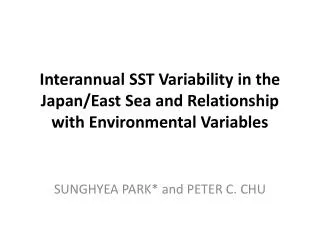
Interannual SST Variability in the Japan/East Sea and Relationship with Environmental Variables SUNGHYEA PARK* and PETER C. CHU
Complex EOF Analysis • Sn(x,y): spatial amplitude and phase • PCn(x,y): temporal amplitude and phase • Fourier Transform • Hilbert Transform • Complex data field • Singular value decomposition • Real / Imaginary
Spatial amplitude and phase • Spatial amplitude An(x, y) distributions (a) and Spatial phase θn(x, y) distributions (b) of each mode. The contour interval of the amplitude is 0.01°C. Signals propagate toward decreasing phase, and contour interval of the phase is 10° (30°) for the first (second) mode.
Spatial and temporal analysis (Left) Spatial amplitude An(x, y) distributions using NOAA Optimum Interpolation Sea Surface Temperature dataset with a horizontal grid of 1° × 1° (contour interval is 0.01°C). (Right) Temporal amplitude Bn(t) variations (a) and temporal phase φn(t) variations (b) of each mode.
Seasonal CEOF Seasonal CEOF. (a) Spatial amplitude (contour interval is 0.01°C), and (b) temporal variation at the grid with a maximum spatial amplitude: (137.5°E, 39.7°N) for the winter first mode, (134.3°E, 41.5°N) for the summer first mode, (128.8°E, 39.4°N) for the winter second mode, and (139.9°E, 46.3°N) for the summer second mode.
Propagation Evolutions of the second mode SSTA over mid-1987~mid-1993 with an interval of 80 days. Phase changes from 360° to 0°. Time instance is recorded as the fraction of a year; e.g., the fraction 1987.5 indicates mid-1987. Contour interval is 0.2°C. Black (white) contours indicate negative (zero and positive) anomaly.
Comparisons to the climate indices • Lag correlation coefficients between the climate indices and the n-th mode JES SSTA, where negative lag indicates that the climate indices lead JES SSTA. (a) First mode, and (b) second mode.