Download
1 / 48
480 likes | 691 Vues
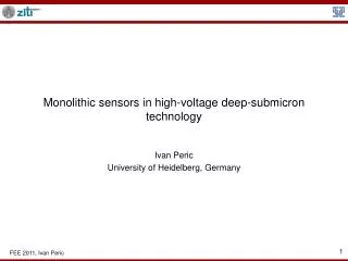
The first beam test of a monolithic particle pixel detector in high-voltage CMOS technology. Ivan Peric, Christian Takacs, Jörg Behr, Franz M. Wagner, Peter Fischer University of Heidelberg. This work draws on the results from an ongoing research project

E N D
The first beam test of a monolithic particle pixel detector in high-voltage CMOS technology Ivan Peric, Christian Takacs, Jörg Behr, Franz M. Wagner, Peter Fischer University of Heidelberg This work draws on the results from an ongoing research project commissioned by the Landesstiftung Baden-Württemberg
Monolithic pixel detectors in high-voltage CMOS technology Main features: Easy to implement (standard CMOS technology used), radiation hard and fast Allow in-pixel signal processing (CMOS) Can be very thin (thinner than 50 μm) Possible applications: particle tracking in the case of high occupancy and harsh radiation environment such as in LHC (upgrade) Introduction
Introduction • First test beam results • First irradiation results DESY CERN (SpS) FRM II
High-voltage monolithic detectors High-voltage monolithic detectors 0V drift <-60V 10 μm tcoll<<100ps • Idea – use high-voltage P/N junctions as sensor • Idea – place the (CMOS) electronics inside the N-well • Collection speed • Radiation hardness diffusion MAPS (as comparison)
High-voltage monolithic detectors High-voltage monolithic detectors drift Rad. damage • Idea – use high-voltage P/N junctions as sensor • Idea – place the (CMOS) electronics inside the N-well • Collection speed • Radiation hardness Rad. damage MAPS (as comparison)
HVD types Binary information Type A Binary readout Analog information Type B Analog readout Rolling shutter addressing Similar to 3D detectors!!! RO chip Analog information Type C Capacitive readout
HVD types Binary information • In-pixel signal processing • Time measurements possible (fast readout) • Leakage current compensation (+ rad. hardnes) Larger pixels Larger capacitance Static current consumption Analog information • Smaller pixels • Smaller capacitance No static current consumption Time measurements not possible Leakage current added to signal (- rad. hardnes) Testbeam!!! RO chip Analog information • Any kind of in-pixel signal processing possible (hybrid detector) • Radiation tolerant layout can be easily implemented Slightly increased noise because of capacitive transmission
Type A 3.3 V CR-RC Comparator FF Bus driver CSA RAM Readout bus 4-bit tune DAC AC coupling 220 fF (50 e ENC measured) N-well 15 μm 40 μm P-substrate -60 V
Type B 2 V 3.3 V Readout bus ResetNWB ResB SelB AC coupling 10 fF (90 e ENC measured) N-well 12 μm 9 μm P-substrate -60 V
Type C Readout chip 3.3 V CR-RC CSA RAM AC coupling 100 fF (system: 80 e ENC measured) – sensor 30 e ENC! N-well 15 μm 35 μm P-substrate -60 V
The “Taki” chip • 128X128 pixel-matrix – pixel size 21X21µm2 • The chip can be easily scaled to 4 or 16 times larger area • Fast digital readout – designed for ~50 s frame readout time (164 s tested) • 128 end-of-column single-slope ADCs with 8-bit precision • Low power design - full chip 55mW (only analog) • Radiation hard design
Chip structure • Pixel size: 21 X 21 m • Matrix size: 2.69 X 2.69 mm (128 X 128) • Possible readout time/matrix: ~50 s (400ns/row) (tested so far 1.28 s/row) • ADC: 8 – Bit • Analog power: 54.9mW (7.63mW/mm2) • Analog power: ADC: 0.363mW/ADC (90μA+10 μA) 10000001000 Pixel matrix Row-control („Switcher“) Amplifier ADC Ramp gen. Comparator 8 LVDS Digital output Counter Latch
ADC • Switched capacitor amplifier • Single slope ADC • Asynchronous 8-bit counter Bricked pixels Guard ring 21 um Ramp Switches S/H Amplifier S/H Amplifier Difference Amplifier Current source Counter Logic Comparator Difference amplifier Pixels
(Problem with the) difference amplifier R2X 4 Amp C4 R1 1 VPLoad UX 2 CX LoadBiasP 6 A2 6 Comp Amp 7 C2 C1 3X 11 R2Y 12 6X 5 10 A1 1 2 3 Input R1 C1 4 5 R3 C3 Amp C6 C5 PDDKS VInput 0 UY 3 CY 0 7 A3 8 9 The amplifier oscillates under standard bias conditions
Noise (present and future) The ENC is mainly caused by the readout electronics Better design Better design 10 e Amplifier Noise : 57 e Follower noise meas : 24 e 10 e DKS Reset noise meas: 65 e Reset noise theory : 42 e 0 e Reducing of ENC from 90 e to 30 e is realistic - > all S/N ratios will be increased by factor 3
Test system • Very simple detector test system – a single PCB • Only 4 external voltages needed, high voltage is generated by batteries • USB 1 communication with DAQ PC Bias voltage “generators” Radioactive s. Power (FPGA) USB FPGA HV Trigger connector Power (det.) 48 MHz
FPGA Frame RO FIFO (frame m.) RAM From TLU cnt Reset values Matrix Row Col ID Cluster readout Ampl R receiver Del receiver S - Rd Wr cmp & Pedestals RAM Th RO FIFO Zero suppresion Pedestal and reset-offset subtraction Pixel detector FPGA PC DKS mode, frame mode- or zero suppressed cluster readout
Test beams with EUDET telescope Test beam DESY DUT EUDET telescope DUT Test beam CERN
Results – MIP signal MIP spectrum (CERN SpS - 120GeV protons) MIP spectrum (60 Co) MIP spectrum (CERN SpS - 120GeV protons) The signal increases from 1200 e (single pixel) to 2200 e (6-pixel cluster) The measured S/N ratio varies from 12.3 (single pixel) to 9.8 (6-pixel cluster)
Results – signal Comparison between60Co and 120GeV proton spectra 60Co signals higher by 10% - expected from theory due to lower particle energy Seed pixel sees about 50% of the total signal The next MSP sees only 25% of the seed pixel signal Cluster size is 6 pixels Moderate charge sharing (the seed gets the most) Do we expect this? – the gaps between n-wells are large, the most of the particles hit the gaps As comparison55Fe Seed pixel sees about 90% of the total signal Cluster size is 3 pixels No charge sharing
Primary and secondary signal (explanation of the measured spectra) Direct hit Hit between the pixels (occurs quite often) P P S1 S3 S1 S2 S3 S2 The drift leads to the primary signal P – this signal portion is not shared between pixels, it is collected in the pixel next to the particle hit point The diffusion of the electrons generated in the non-depleted bulk is the secondary signal mechanism P measured with type A det. – good agreement S2 S1 P
Is there sharing of primary signal? Do we have gaps with zero E-field? (Moreover, they could be insensitive to particles) Is there sharing of primary signal? Such clusters could be lost after applying the seed cut…
Fe-55 (explanation of the measured spectra) No charge sharing A small part of the signal is seen by the next pixel Seen very seldom Seen very seldom
Gap investigation Do we have gaps with zero E field? If yes, there will be a certain number of clusters with two equal seeds COG correction should be then 0.5 pixel size
CoG correction distribution in pixel frame of reference The COG correction distribution is not homogenous inside a pixel due to reduced charge sharing – the small CoG correction values occur more frequently Large CoG values occur very seldom => there are no sensitive gaps with E=0 but… the gaps could be insensitive Or the clusters with two equal seeds could be lost after applying the seed cut… Number of clusters Pixel centre: (0.0105, 0.0105) In-pixel CoG coordinate [mm]
Efficiency Efficiency is the answer but… Efficiency is homogenous over the matrix area and saturates at 86%for low seed/cluster thresholds Efficiency Seed and cluster cut [SNR]
Track and system geometry Telescope planes DUT Scintillator Scintillator
(Irregular events) double track event Out of time track – not seen by DUT In time track – seen by DUT Readout times “taki” “Mimotel” T (trigger) 160 800 T [μs] 0
(Irregular events) empty event In time track – not seen by Mimotel Readout times “taki” Mimotel T (trigger) 160 800 T [μs] 0
(Irregular events) double track event seen as a single track event In time track – not seen by Mimotel Out of time track – not seen by DUT Readout times “taki” Mimotel T (trigger) 160 800 T [μs] 0
Efficiency (conclusions) • Efficiency lower than 100% probably due to timing issues • Readout of telescope and DUT are not synchronous • DUT integration (readout) time 164 μs • Telescope integration time = 800 μs • Large cluster and track multiplicity in telescope • multiple tracks in telescope due to high beam intensity and long integration time • Small cluster multiplicity in DUT due to shorter integration time • Some “out of time” particles hit the telescope after the trigger moment (during the readout) – the particles are not seen by the DUT due to wrong timing • Neglecting of all multiple track events increases efficiency from 72% to 86% • Problem: A part of scintillator outside the telescope area: some out of time tracks are seen as single tracks by telescope. If we were able to filter these out of time tracks too, we would probably measure a better efficiency
In-pixel measurements – back-propagation Back-propagation Alignment Excellent spatial resolution of the EUDET telescope allows the investigation of DUT properties as function of the in-pixel hit point We performed series of such n-pixel measurements The fitted coordinate is back-propagated to the DUT frame of reference and DUT pixels frame of reference
In-pixel CoG • CoG correction works but the slope is too small (by factor ~ 3) probably due to absence of charge sharing (primary signal) and noise (Eta-correction does not lead to better results) • Good check of the back-propagation tool In-pixel position Pixel centre: 0.0105 mm
In-pixel efficiency There are no insensitive regions! => There are no E=0 gaps! In-pixel position Pixel centre: (0.0105, 0.0105)
Spatial resolution • Spatial resolution • Sigma residual X: 7.3 μm • Sigma residual Y: 8.6 μm • The difference is probably caused by the bricked pixel geometry – still not understood completely, simulations will be done • The spatial resolution is not as good as in the case of standard MAPS due to absence of charge sharing in the case of primary signal • It is not completely clear why is the resolution worse than 21 μm /sqrt(12) = 6.1 μm • The residual is sometimes larger than the pixel pitch.
Seed pixel – fitted hit point mismatch • The back-propagation (in pixel measurements) show that the fitted hit point (measured by the telescope) is sometimes outside (in the next pixel) of the seed pixel. • This mismatch worsens the spatial resolution • The fitted hit point – seed pixel mismatch occurs more probably when fitted point is near the pixel boundary • The mismatch seems, however, not to be caused by the electronic noise
Seed pixel – fitted point mismatch (clusters and their pixel S/N) A few clusters when the fitted point is outside the seed pixels are shown – the seed pixel amplitude (S/N amplitude) is always very high – there is little chance that we have chosen the wrong seed due to electronic noise. 6.1 2.3 3.4 2.5 2.2 2.9 5.1 10 6.0 49 14.0 1.2 11 0.0 2.8 55 3.4 1.6 37 4.6 13 27 -2.5 1.3 3.8 1.9 2.2 0.2 4.2 6.4 3.8 3.2 2.5 3.2 1.3 -0.8 0.4 15 4.2 3.0 30 3.4 4 27 1.6 2.7 28 1.8 1.3 0.8 0.6 3.5 3.2 3.9 3.1 2.1 -0.2 6.5 2.4 0.9 1.4 2.7 -0.8 3.3 -0.3 20 4.0 1.4 23 4.6 4.8 17 4.0 2.0 33 0.7 1.0 1.3 0.2 0.7 0.6 1.8 5.9 5.0
Seed pixel – fitted point mismatch The mismatch seems to be caused by the measurement-setup uncertainties, e.g. mechanical instability, multiple scattering on PCB “vias”. real track fitted predicted error Chip Cu 1.3mm Via PCB
Summary (test beam) • Efficiency: 86% • Purity: 72% • Sigma X-residual 8.6 μm • Sigma Y-residual 7.3 μm • S/N ratio seed: 12.3 • S/N ratio cluster (6 pixels): 10 • There is little charge sharing – the seed pixel receives 50 % or more of the total signal • There are no insensitive regions • Spatial resolution worse than expected probably due to MS, to be understood
Irradiation Irradiation with neutrons has been performed by Franz M. Wagner at FRM II - “Forschungsneutronenquelle Heinz-Maier-Leibnitz” http://www.frm2.tum.de/
Irradiation with neutrons (1014 neq) – signal (Type A) After irradiation to 1014 neq the seed “MIP” (most probable 60Co) signal is 1000 e and the cluster signal is 1300 e – the real MIP is by about 10% lower The measurement has been performed at 0C Leakage current / pixel increases from 350 fA to 130 pA Not irradiated Irradiated
Irradiation with neutrons (1014 neq) – noise (Type C) • Type C detector, 55Fe spectrum • Excellent noise performance after irradiation • No clustering possible with this detector Irradiated to 1014 neq,- 30C, noise about 30 e Irradiated to 1014 neq,room temperature, noise about 60 e
Summary Type B (10 fF detector capacitance, 21 μm x 21 μm pixel size) • Signal: • not irradiated: 1200 e (seed) to 2200 e (cluster) (MIP) • Irradiated to 1014 neq : 1000 e (seed) to 1300 e (cluster) (60Co) • Noise: 90 e (not irradiated) – the high noise is the result of non-optimal design, will be reduced by new design (the chip has already been submitted) • Type A (220 f detector capacitance, 55 μm x 55 μm pixel size) • Signal: • Not irradiated: 1700 e (MIP) (good agreement with type B) • Noise 55 e at 110 ns shaping time • Extrapolations for type A: • Signal after 1014 : 1200 e (MIP) • Signal after 1015 : 800 e • Type C (100 f detector capacitance, 50 μm x 50 μm pixel size) • Noise after 1014 neq : 60 e (longer shaping times) (room T) • Radiation hardness of more than 2 MRad tested • Future plans: irradiation to at least 1015 neq and 50 MRad