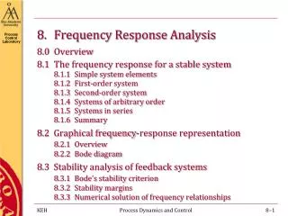
Frequency Response Analysis Methods
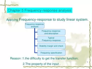
Learn about frequency response analysis and how to study a system's steady-state response to sinusoidal inputs by varying signal frequencies. Explore advantages, steady-state outputs, transfer functions, and design principles. Understand Bode diagrams and practical applications in control systems.


Frequency Response Analysis Methods
E N D
Presentation Transcript
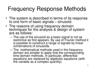
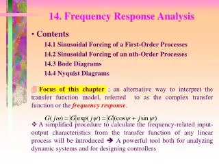
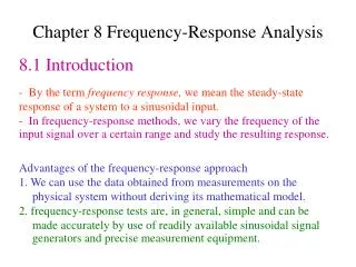
Frequency-Response Analysis Introduction - By the term frequency response, we mean the steady-state response of a system to a sinusoidal input. - In frequency-response methods, we vary the frequency of the input signal over a certain range and study the resulting response. Advantages of the frequency-response approach 1. We can use the data obtained from measurements on the physical system without deriving its mathematical model. 2. frequency-response tests are, in general, simple and can be made accurately by use of readily available sinusoidal signal generators and precise measurement equipment.
Advantages of the frequency-response approach (ต่อ) 3. The transfer functions of complicated components can be determined experimentally by frequency-response tests. 4. A system may be designed so that the effects of undesirable noise are negligible and that such analysis and design can be extended to certain nonlinear control systems. In designing a closed-loop system, we adjust the frequency-response characteristic of the open-loop transfer function by using several design criteria in order to obtain acceptable transient-response characteristics for the system.
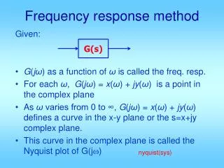
Obtaining Steady-State Outputs to Sinusoidal Inputs • The steady-state output of a transfer function system can be obtained directly from the sinusoidal transfer function, that is, the transfer function in which s is replaced by j, where is frequency. Figure 8-1 Stable, linear, time-invariant system. - If the input x(t) is a sinusoidal signal, the steady-state output will also be a sinusoidal signal of the same frequency, but with possibly different magnitude and phase angle.
Obtaining Steady-State Outputs to Sinusoidal Inputs • The steady-state output of a transfer function system can be obtained directly from the sinusoidal transfer function, that is, the transfer function in which s is replaced by j, where is frequency. x(t)= X sin t Steady-state response
The partial fraction expansion of Equation (8-1) The inverse Laplace transform of Equation (8-2) The steady-state response
Figure 8-2 Input and output sinusoidal signals. Sinusoidal transfer fn. ได้มาจากการแทนค่าs ด้วยj
The curves are drawn on semilog paper, using the log scale for frequency and the linear stale for either magnitude (but in decibels) or phase angle (in degrees). The main advantage of using the Bode diagram 1. Multiplication of magnitudes can be converted into addition. 2. A simple method for sketching an approximate log-magnitude curve is available. 3. It is based on asymptotic approximations. 4. The experimental determination of a transfer function can be made simple if frequency-response data are presented in the form of a Bode diagram.
1. A number greater than unity has a positive value in decibels, while a number smaller than unity has a negative value. 2. The log-magnitude curve for a constant gain K is a horizontal straight line at the magnitude of 20 logK decibels. 3. The phase angle of the gain K is zero. 4. The effect of varying the gain K in the transfer function is that it raises or lowers the log-magnitude curve of the transfer function by the corresponding constant amount, but it has no effect on the phase curve.
- In Bode diagrams, frequency ratios are expressed in terms of octaves or decades. - An octave is a frequency band from 1to 21 - A decade is a frequency band from 1to 101
- The phase angle of jis constant and equal to 90°. - The log-magnitude curve is a straight line with a slope of 20 dB/decade.
Figure 7-5 (a) Bode diagram of G(jω) = 1/jω; (b) Bode diagram of G(jω) = jω.
Thus, the value of -20 log T dB decreases by 20 dB for every decade of - At = 1/T, the log magnitude equals 0 dB. - At = 10/T, the log magnitude is -20 dB. For »1/T, the log-magnitude curve is thus a straight line with a slope of -20 dB/decade (or -6 dB/octave).
Figure 8-6 Log-magnitude curve, together with the asymptotes, and phase-angle curve of 1/(1+jωT).
The error at one octave below or above the corner frequency is approximately equal to -1 dB. Similarly, the error at one decade below or above the corner frequency is approximately -0.04 dB.
Figure 8-7 Log-magnitude error in the asymptotic expression of the frequency-response curve of 1/(1+jωT).
In practice, an accurate frequency-response curve can be drawn by introducing a correction of 3 dB at the corner frequency and a correction of 1 dB at points one octave below and above the corner frequency and then connecting these points by a smooth curve. Note that varying the time constant T shifts the corner frequency to the left or to the right, but the shapes of the log-magnitude and the phase-angle curves remain the same. • The transfer function 1/(1 + jT) has the characteristics of a low-pass filter. • Therefore, if the input function contains many harmonics, then the low-frequency components are reproduced faithfully at the output, while the high frequency components are attenuated in amplitude and shifted in phase.
An advantage of the Bode diagram is that for reciprocal factors-for example, the factor 1 + jT-the log-magnitude and the phase-angle curves need only be changed in sign, since
Figure 8-8 Log-magnitude curve, together with the asymptotes, and phase-angle curve for 1+jωT.
If > 1, this quadratic factor can be expressed as a product of two first-order factors with real poles. • If 0 < < 1, this quadratic factor is the product of two complex conjugate factors.
Errors obviously exist in the approximation by straight-line asymptotes. The magnitude of th error depends on the value of .
Figure 7-9 Log-magnitude curves, together with the asymptotes, and phase-angle curves of the quadratic transfer function given by Equation (8–7).
First rewrite the sinusoidal transfer function G(j)H(j) as a product of basic factors discussed above. • Then identify the corner frequencies associated with these basic factors. • Finally, draw the asymptotic log-magnitude curves with proper slopes between the corner frequencies. • The exact curve, which lies close to the asymptotic curve, can be obtained by adding proper corrections. • The phase-angle curve of G(j)H(j) can be drawn by adding the phase-angle curves of individual factors.
Figure 7-11 Bode diagram of the system considered in Example 7–3.