8 . Frequency Response Analysis
8 . Frequency Response Analysis. 8.0 Overview 8.1 The frequency response for a stable system 8.1.1 Simple system elements 8.1.2 First-order system 8.1.3 Second-order system 8.1.4 Systems of arbitrary order 8.1.5 Systems in series 8.1.6 Summary

8 . Frequency Response Analysis
E N D
Presentation Transcript
8. Frequency Response Analysis 8.0 Overview 8.1 The frequency response for a stable system 8.1.1Simple system elements 8.1.2 First-order system 8.1.3 Second-order system 8.1.4 Systems of arbitrary order 8.1.5 Systems in series 8.1.6Summary 8.2 Graphical frequency-response representation 8.2.1Overview 8.2.2 Bode diagram 8.3 Stability analysis of feedback systems 8.3.1Bode’s stability criterion 8.3.2 Stability margins 8.3.3 Numerical solution of frequency relationships Process Dynamics and Control
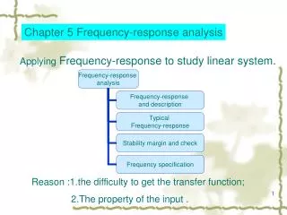
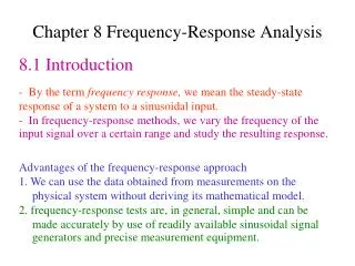
8.0 Overview • So far in this course system properties have been studied in the • time domain (e.g., step response) • Laplace domain (e.g., stability) • In this chapter, system properties are studied in the • frequency domain • by studying the stationary behaviour when the system is excited by a sinusoidal input of given frequency. Stationary behaviour refers to the situation when initial effects have vanished, i.e., when the time . • The output from a linear system will then also change sinusoidally with certain characteristic properties that depend on the system as well as the amplitude and frequency of the input sinusoidal. These properties expressed as function of the input frequency are referred to as the frequency response of the system. System analysis based on the frequency response is called frequency analysis. • The study of sinusoidal inputs is useful because measurement noise and time-varying disturbances can often be approximated by sinusoidal signals. Process Dynamics and Control
8.1 The frequency response for a stable system • In this section, the frequency response for an arbitrary linear, stable, system is derived. • In order to introduce new concepts step-wise, some simple system elements that essentially lack dynamics are treated first. These elements are often part of more complex systems. • After this, systems of first and second order are considered. In these systems, dynamics play a prominent role. • For the derivation of the frequency response of high-order systems, the frequency response of simpler systems is utilized. The decompo-sition of a high-order system into low-order components connected in series is fundamental in frequency analysis. Process Dynamics and Control
8.1 Frequency response for a stable system 8.1.1 Simple system elements • Static system • A linear static system is described by • (8.1) • where is an input, is an output, and is the system gain. Let the input change sinusoidally as • (8.2) • where is the angular frequency (expressed in radians per time unit) and is the amplitude of the sinusoidal. The output is then • (8.3) • There are now two situations regarding the phase of the output: • If , it is the same as the phase of the input. • If , it is opposite to the phase of the input. In this case, has a maximum when has a minimum, and vice versa. • Thus, the negative system gain causes a phaseshift of radians, or in the output. Process Dynamics and Control
Static system • It is of interest to rewrite (8.3) so that • the phase shift is explicitly seen in the equation • the output amplitude is always a positive quantity • To accomplish this, (8.3) is written as • (8.4) • where • (8.5) • is the phase shift of the system. • The ratio between the amplitudes of the output and input signals is also of interest. In this case, the amplitude ratio is • (8.6) • Generally, the output can be written as • (8.7) • The stationary output of any stable linear system with an input (8.2) can be written as (8.7), where is the amplitude ratio and is the phase shift of the system in question. Process Dynamics and Control
8.1.1 Simple system elements • Derivative system • A system with the transfer function has an output that is the time derivative of the input amplified by the factor , i.e., • (8.8) • When the input is sinusoidal as in (8.2), the output becomes • (8.9) • where the relationship has been used. • Here the output is a cosine function, but by using the trigonometric identity , (8.9) can be written as • (8.10) • Here the phase shift is used, not , although they both give the same output. The reason is not that is closer to 0, but that the derivative yields a prediction of the input. Hence, the output can be considered to correspond to a future value of the input meaning that the phase of the output is before the phase of the input. Thus, the derivative is a phase-advancing element. Process Dynamics and Control
Derivative system • If the gain , this has to be taken into account as for a static system. Thus, the output is given by (8.7) with • (8.11) • (8.12) • Parallel connection of static and derivative system • A system composed of a parallel connection of a static and a derivative system has the transfer function • (8.13) • This can be a PD controller, but other systems with zeroes also have such factors in the numerator of the transfer function. • In the time domain, the output is given by • (8.14) • When the input is a sinusoidal as in (8.2), this gives • (8.15) Process Dynamics and Control
Parallel connection of static and derivative system • The right-hand side of (8.15) can be written as a single sine function by means of the trigonometric identity • (8.16) • This gives • (8.17) • The output is thus given by (8.7) with • (8.18) • (8.19) • Note that the function is the same function as . Process Dynamics and Control
8.1.1 Simple system elements • Integrating system • A system with the transfer function has an output that is the time integral of the input amplified by the factor . This is equivalent to the time derivative of the output being equal to the input amplified by , i.e., • (8.20) • The sinusoidal input (8.2) gives • (8.21) • Because , it is easy to verify by differentiation that • (8.22) • satisfies (8.20). Substitution of into (8.22) yields, with the sign of taken into account, (8.7) with • (8.23) • (8.24) Process Dynamics and Control
Integrating system • Parallel connection of static and integrating system • A system composed of a parallel connection of a static and an integrating system has the transfer function • (8.25) • This can, e.g., be the transfer function of a PI controller. From (8.3) and (8.22) it is clear that the sinusoidal input (8.2) gives • (8.26) • Taking the trigonometric identity (8.16) and the sign of into account yields (8.7) with • (8.27) • (8.28) Process Dynamics and Control
8.1.1 Simple system elements • Time delay • A time delay of length has the transfer function . In the time domain, the relationship between the output and the input is • (8.29) • The sinusoidal input (8.2) then gives • (8.30) • where • (8.31) • As seen from (8.30), a pure time delay has the amplitude ratio • (8.32) • Note that the phase shift of a time delay is unlimited — the higher the frequency, the more negative the phase shift. Process Dynamics and Control
8.1 Frequency response for a stable system 8.1.2 First-order system • A first-order system is described by the differential equation • (8.33) • where is an input, is an output, is the gain, and is the time constant of the system. • Frequency response via the Laplace domain • As for the previous cases, the frequency response could be derived directly in the time domain. However, • it is instructive to derive the frequency response via the Laplace domain; • this will help derive more general relationships for the frequency response, • which are useful when systems of arbitrary order are considered. Process Dynamics and Control
Frequency response via the Laplace domain • Laplace transformation of (8.33) yields • , (8.34) • where is the Laplace transform of , is the Laplace transform of , and is the transfer function of the system. The Laplace transform of the sinusoidal input (8.2) is • (8.35) • which substituted into (8.34) gives • (8.36) • Since the second-order factor has complex-conjugated zeroes, (8.36) has the partial fraction expansion • (8.37) • where the coefficients , and have to be determined so that (8.36) and (8.37) are equivalent. Process Dynamics and Control
Frequency response via the Laplace domain • It is useful to consider the inverse Laplace transform of (8.37) before , and are determined. The transforms 25, 38 and 39 in the Laplace transform table in Section 4.5 yield • (8.38) • We are interested in the stationary solution when . Because for a stable system, and is finite, the first term on the right-hand side will vanish as . Thus, the stationary solution is • (8.39) • This means that the coefficient does not affect the stationary solution and it is sufficient to determine only and if it can be done indepen-dently of . • Combination of the first part of (8.36) with (8.37) gives • from which • (8.40) Process Dynamics and Control
Frequency response via the Laplace domain • The identity (8.40) has to apply for arbitrary values of . Choosing means that . Then (8.40) yields • (8.41) • The identity (8.41) requires that the real part and the imaginary part are satisfied independently. Because is a complex number with the real part and the imaginary part , i.e., • (8.41) yields • , (8.42) • The first-order system (8.34) yields • (8.43) • from which • , (8.44) Process Dynamics and Control
Frequency response via the Laplace domain • Substitution of (8.44) into (8.42) and further into (8.39) yields the stationary solution • (8.45) • The trigonometrical identity (8.16) applied to (8.45) yields • (8.46) • Thus, the stationary solution has the same form as (8.7), i.e., • (8.47) • For a first-order system (8.47) applies with • (8.48) • (8.49) Process Dynamics and Control
8.1 Frequency response for a stable system 8.1.3 Second-order system • A second-order system without zeroes and with no time delay has the transfer function • (8.50a) • where is the static gain of the system, is its relative damping and is its undamped natural frequency. Since only stable systems are considered, . If the poles of the system are real, the transfer function is often written in the form • (8.50b) • The parameters of (8.50a) are then given by • , (8.51) • It is here sufficient to consider second-order systems without zeroes be-cause systems with zeroes can be decomposed into a series connection of two (or more) subsystems and handled by the methods in Section 5.1.5. Process Dynamics and Control
8.1.3 Second-order system • Derivation of frequency response • Analogously to (8.36), the Laplace transform of the sinusoidal input yields • (8.52) • When , there always exists a partial fraction expansion • (8.53) • According to our Laplace transform table, the first term on the right-hand side has an inverse transform containing the factor , where denotes time. Because , as and the term containing this factor will vanish. • This means that also in this case • the stationary solution to (8.53) is given by (8.39) • the coefficients and are given by (8.42) Process Dynamics and Control
Derivation of frequency response • In this case • (8.54) • from which • , (8.55) • Substitution into (8.42) and further into (8.39) gives • (8.56) • where we (for now) assume that . Application of the trigono-metric identity (8.16) now yields the stationary response as • , (8.57) Process Dynamics and Control
Derivation of frequency response • Eq. (8.57) can be expressed in the form of (8.47) with • (8.58) • (8.59a) • (8.59b) • For , these reduce to • , , (8.60–61) • If , the amplitude ratio has a peak (i.e., maximum) at the peak frequency, given by • (8.62–63) Process Dynamics and Control
8.1 Frequency response for a stable system 8.1.4 Systems of arbitrary order • For a stable system of arbitrary order, but no time delay, the response to a sinusoidal input can be expressed by a partial fraction expansion as in (8.37) and (8.53). As before, the stationary solution in the time-domain is given by (8.39) with and given by (8.42). • To simplify the notation, we define • , (8.64) • Substitution of (8.42) into (8.39) then gives • (8.65) • Application of the trigonometrical identity (8.16) yields • (8.66) • where • (8.67) Process Dynamics and Control
8.1.4 Systems of arbitrary order • Because is a complex number, it can be characterized by its magnitude and argument, also denoted . According to the theory of complex number, • , (8.68a,b) • The sign of in (8.66) has the same effect on the phase shift as the sign of the gain in previous sections. Substitution of (8.68) into (8.66) and (8.67) then yields • (8.69) • (8.70) • From (8.69) it is obvious that • the magnitude is identical to the amplitude ratio • the argument is identical to the phase shift • Thus • , (8.71) Process Dynamics and Control
8.1.4 Systems of arbitrary order • Because the function only takes values between and , direct calculation from (8.70) gives an argument in the range • (8.72) • However, because of the periodicity of the trigonometric functions, (8.68b) would be satisfied for any integer multiple of added to This means that the solution calculated from (8.70) is ambiguous by an integer multiple of . • The figure shows a sinusoidal input and the stationary output , which is also sinusoidal. When the axes are normalized as indicated, the values of and can be directly read • from the plot for the applied • input frequency. Because the • sinusoidal signals can be • shifted by an integer multiple • of without any detectable • difference, is similarly • ambiguous also here. • This ambiguity can be solved • by the method in Section 5.1.5. Process Dynamics and Control
8.1 Frequency response for a stable system 8.1.5 Systems in series • Consider a system composed of subsystems connected in series. If the subsystems have the transfer functions , , the transfer function of the full system is given by • (8.73) • Conversely, a system with the transfer function • (8.74) • can be decomposed into the series-connected subsystems • , , ,…, , ,…, , . • If the system has complex-conjugated poles or zeroes, they can be included as second-order factors in the decomposition. • Thus, a high-order transfer function can be decomposed into factors of at most second order and a possible time delay. Process Dynamics and Control
8.1.5 Systems in series • From (8.73) it follows that the frequency response of the full system is • (8.75) • where , , are the frequency responses of the individual subsystems. • According to the theory of complex numbers, can be expressed in terms of its magnitude and its argument as • (8.76) • Substitution into (8.75) yields • (8.77) • Naturally, can also be expressed as (8.76). From that and (8.77) • (8.78) • (8.79) Process Dynamics and Control
8.1.5 Systems in series • Equations (8.78) and (8.79) mean that for the full system the • amplitude ratio (or magnitude) is obtained as the product of the amplitude ratios (or magnitudes) of the subsystems • phase shift (or argument) is obtained as the sum of the phase shifts (or arguments) of the subsystems • The user is allowed to decompose the full system into subsystems as desired. However, it is advantageous to decompose into subsystems of first or second order and a possible time delay because we know the frequency responses of such systems. In particular, we know that • a first-order system has a phase shift in the range • a second-order system has a phase shift in the range • By adding up the phase shifts (arguments) of the individual subsystems according to (8.79), the correct phase shift (argument) for the full system is obtained. This means that a phase shift outside the range of (8.72) can be obtained, i.e., the correct integer multiple of is obtained. Process Dynamics and Control
8.1 Frequency response for a stable system 8.1.6Summary • Table 8.1. Frequency response of low-order systems. Process Dynamics and Control
8.2 Graphical frequency-response representation • 8.2.1 Overview • The complex-valued function of a system with the transfer function contains all information about the frequency response of the system—except for a multiple of in the phase shift. • can be considered a system property • is called the frequency function • Since is a complex number, it can be represented in two ways: • is the real part of • is the imaginary part of • is the magnitude of • is the argument of This gives several possibilities of representing graphically, e.g., • Nyquist diagram: vs as varies • Bode diagram: vs and vs in two diagrams Process Dynamics and Control
8.2 Graphical representations 8.2.1 Nyquist diagram • The Nyquist diagram is a graphical • representation of in the • complex plane. • For a given angular frequency , is a point in the complex plane. • When the frequency varies, the points of produce a curve. • When the frequency varies from Fig. A point in the to , the curve is called a complex plane. frequency plot also known as a Nyquist plot. Process Dynamics and Control