Frequency Response
Frequency Response. Last time we Discussed the possibility of representing signals as sums of sinusoids (known as Fourier series) Had MATLAB calculate Fourier series coefficients for example signals Today we will Revisit formal definitions of linearity and time-invariance


Frequency Response
E N D
Presentation Transcript
Frequency Response Last time we • Discussed the possibility of representing signals as sums of sinusoids (known as Fourier series) • Had MATLAB calculate Fourier series coefficients for example signals Today we will • Revisit formal definitions of linearity and time-invariance • Find an eigenfunction for linear time-invariant systems • Find the frequency response of a linear system EECS 20 Chapter 8 Part 1
Continuous Linear Time-Invariant Systems Consider a continuous system S with the description S: [Reals→Complex] → [Reals→Complex] S takes complex-valued time functions as input, and outputs complex-valued time functions. Let’s look at the special case when S is linear. Recall that this means S satisfies the following properties: For all x [Reals→Complex] and for all a Complex, S(ax) = a S(x) homogeneity and For all x1, x2 [Reals→Complex] S(x1+x2) = S(x1) + S(x2) additivity EECS 20 Chapter 8 Part 1
Continuous Linear Time-Invariant Systems Let’s look at the further special case where S is linear and time-invariant. S is time-invariant means that the output depends only on the value of the input, not when it is applied. Consider the delay system D, where the output is equal to the input delayed by : • x [Reals→Complex] and t Reals, D(x)(t) = x(t- ) We may define time invariance for any continuous system using this delay system. We say S is time-invariant if • Reals, S D = D S A system S is time invariant, if, for any input x producing output y, the delayed input D(x) produces the delayed output D(y). EECS 20 Chapter 8 Part 1
Eigenfunction Our LTI system S can take any complex-valued function of time as input. For certain special inputs called eigenfunctions, the output will be a scaled version of the input. The output will be the same “kind” of function as the input; just with a scaling factor. Consider inputs which are complex exponentials, having the form x(t) = eiωt for all t Reals, where ω is a real parameter called the frequency. This term comes from the fact that EECS 20 Chapter 8 Part 1
Eigenfunction What is the output S(x) for an input x of this form? We know that S(D(x)) = D(S(x)) and for a complex exponential input, D(x)(t) = eiω(t-) = e-iω eiωt = e-iω x(t) Since e-iω is a constant we can pull out, we may write e-iωS(x) = D(S(x)) EECS 20 Chapter 8 Part 1
Eigenfunction For convenience, let’s express S(x) as y: e-iωy(t) = D(y)(t) = y(t-) Since this is true for all t Reals, we consider the special case when t = 0, e-iωy(0) = y(-) and make a variable substitution s = - (so s is any real number) eiωsy(0) = y(s) So the output y has the same form as the input x, just multiplied by the constant y(0). Thus, eiωt is an eigenfunction of S. EECS 20 Chapter 8 Part 1
Frequency Response This constant y(0) will depend on the input parameter ω. (We know that y(0) cannot depend on t since the system is time-invariant). Thus, we give y(0) the special name H(ω): y(t) = H(ω) eiωt This H(ω) is called the frequency response of the system. It tells us how much the system will scale a complex exponential input of frequency ω. We can prove the same statements for discrete LTI systems. For an LTI system T: [Integers→Complex] → [Integers→Complex] • n Integers, y(n) = H(ω) eiωn EECS 20 Chapter 8 Part 1
Finding the Frequency Response To find the frequency response H(ω) for a system, we can: • Put in the input x(t) = eiωt • Find the corresponding output y(t) • Factor out the eiωt present in the expression for y(t) • The multiplier on eiωt is the frequency response H(ω) EECS 20 Chapter 8 Part 1
Example Consider the two-point moving average system: y(n) = (x(n) + x(n-1)) / 2 Find H(ω) for this system. Let x(n) = eiωn. We can write y(n): y(n) = (eiωn + eiω(n-1)) / 2 y(n) = eiωn (1+ e-iω) / 2 Therefore, H(ω) = (1+ e-iω) / 2 Note that for the delay system D, H(ω) = e-iω. EECS 20 Chapter 8 Part 1
Block Diagram Visualization A block diagram makes it easy to see how we get H(ω) for this system. We can break up the moving average formula into parts and see how they combine: H(ω) = (1+ e-iω) / 2 x + y Divide by 2 H(ω) = 1/2 Delay by 1 H(ω) = e-iω + EECS 20 Chapter 8 Part 1
Cascade Connection When we cascade two LTI systems, y = H2(ω) (H1(ω) x) = H2(ω) • H1(ω) • x = H1(ω) • H2(ω) • x the composite frequency response is the product of the two individual frequency responses: x y S1 S2 Since multiplication of complex numbers is commutative, the composite system is the same when the order of the individual systems is reversed: x y S2 S1 EECS 20 Chapter 8 Part 1
Feedback Connection Consider the feedback connection: We see that y = H1(ω) (x + H2(ω) y) y - H1(ω) H2(ω) y = H1(ω) x This is often called Mason’s Rule. x + y S1 + S2 EECS 20 Chapter 8 Part 1
Difference Equations The moving-average system is a specific example of a difference equation. Difference equations have the form: a0y(n) + a1y(n-1) + … + aNy(n-N) = b0x(n) + b1x(n-1) + … + bMx(n-M) We know that the delay system D has response e-iω so: a0H(ω)x + a1e-iωH(ω)x + … + aNe-iNωH(ω)x = b0x + b1e-iωx + … + bMe-iMωx This means H(ω) is a ratio of polynomials in e-iω: EECS 20 Chapter 8 Part 1
Another Example R Consider the series RC circuit: This circuit is governed by the differential equation Notice that so we may write leading to + + x(t) y(t) C _ _ Low Pass Filter! EECS 20 Chapter 8 Part 1
Differential Equations We just saw that the derivative operator has frequency response H(ω) = iω . So for a general linear differential equation we may write This means H(ω) is a ratio of polynomials in iω: EECS 20 Chapter 8 Part 1
Preview Why are we doing all this work just to find out how the output depends on the frequency of this particular type of input? Does this analysis give us any insight into the output obtained from a general input? Recall that cosines can be expressed as complex exponentials, and that any signal can be expressed as sums of cosines, This analysis will eventually give us insight into the output behavior for any general input, and let us design systems. EECS 20 Chapter 8 Part 1