Frequency Response Methods
Frequency Response Methods. SYSTEMS AND CONTROL I ECE 09.321 11/19/07 – Lecture 17 ROWAN UNIVERSITY College of Engineering Prof. John Colton DEPARTMENT OF ELECTRICAL & COMPUTER ENGINEERING Fall 2007 - Semester One. Some Administrative Items.

Frequency Response Methods
E N D
Presentation Transcript
Frequency Response Methods SYSTEMS AND CONTROL I ECE 09.321 11/19/07 – Lecture 17 ROWAN UNIVERSITY College of Engineering Prof. John Colton DEPARTMENT OF ELECTRICAL & COMPUTER ENGINEERING Fall 2007 - Semester One
Some Administrative Items • Quiz 4 results: mean 75.0, SD 9.7 • Quiz 5 will be on Wednesday 11/28 9:50 AM to 10:40 AM. • Problem Set 11 is due 11/21 • Lab Project 4 Report is due today • Lab Project 5 is conducted today
Stability of Linear Feedback Control Systems • Stability Defined • Routh – Hurwitz Stability Criterion • Root Locus • Frequency Response Methods • Gain and phase margin • Nyquist Criterion
Frequency Response Methods • Frequency Response • Polar Plots • Bode Plots • Performance Specifications in the frequency domain • Examples
LTI System x(t) X(s) y(t) Y(s) H(s) h(t) y(t) = x(t) * h(t) Y(s) = H(s) X(s) where y(t) ↔ Y(s) x(t) ↔ X(s) h(t) ↔ H(s) Laplace transforms and LTI system behavior
Frequency Response of an LTI System The frequency response of a stable linear time-invariant system is defined as the steady-state response of the system to a sinusoidal input signal. Since e st is an eigenfunction of an LTI system, if x(t) = e stis input to such a system, the output of that system is given by y(t) = H(s) e st for any complex frequency s = σ + jω H(s) is called the eigenvector of the LTI system Letting s = jω, we obtain a sinusoidal input x(t) = e jωt = cos ωt + j sin ωt If a sinusoidal signal A cos ω0 t or B sin ω0 t or Ce jω0t is input to an LTI system, the frequency of the output as well as signals throughout the system is sinusoidal in the steady state at frequency ω0 ,differing from the input signal only in amplitude and phase angle. e jω0t → H(jω0 ) e jω0t = │H(jω0 ) │e j H(jω0) e jω0t So the steady state output signal depends only on the magnitude and phase of H(j ω0 ) at a specific frequency ω0
Frequency Response of an LTI System The frequency response of a stable linear time-invariant system is defined as the steady-state response of the system to a sinusoidal input signal. Since e st is an eigenfunction of an LTI system, if x(t) = e stis input to such a system, the output of that system is given by y(t) = H(s) e st for any complex frequency s = σ + jω H(s) is called the eigenvector of the LTI system Letting s = jω, we obtain a sinusoidal input x(t) = e jωt = cos ωt + j sin ωt If a sinusoidal signal A cos ω0 t or B sin ω0 t or Ce jω0t is input to an LTI system, the frequency of the output as well as signals throughout the system is sinusoidal in the steady state at frequency ω0 ,differing from the input signal only in amplitude and phase angle. e jω0t → H(jω0 ) e jω0t = │H(jω0 ) │e j H(jω0) e jω0t So the steady state output signal depends only on the magnitude and phase of H(j ω0 ) at a specific frequency ω0
Frequency Response of an LTI System The frequency response of a stable linear time-invariant system is defined as the steady-state response of the system to a sinusoidal input signal. Since e st is an eigenfunction of an LTI system, if x(t) = e stis input to such a system, the output of that system is given by y(t) = H(s) e st for any complex frequency s = σ + jω H(s) is called the eigenvector of the LTI system Letting s = jω, we obtain a sinusoidal input x(t) = e jωt = cos ωt + j sin ωt If a sinusoidal signal A cos ω0 t or B sin ω0 t or Ce jω0t is input to an LTI system, the frequency of the output as well as signals throughout the system is sinusoidal in the steady state at frequency ω0 ,differing from the input signal only in amplitude and phase angle. e jω0t → H(jω0 ) e jω0t = │H(jω0 ) │e j H(jω0) e jω0t So the steady state output signal depends only on the magnitude and phase of H(j ω0 ) at a specific frequency ω0
Frequency Response of an LTI System The frequency response of a stable linear time-invariant system is defined as the steady-state response of the system to a sinusoidal input signal. Since e st is an eigenfunction of an LTI system, if x(t) = e stis input to such a system, the output of that system is given by y(t) = H(s) e st for any complex frequency s = σ + jω H(s) is called the eigenvector of the LTI system Letting s = jω, we obtain a sinusoidal input x(t) = e jωt = cos ωt + j sin ωt If a sinusoidal signal A cos ω0 t or B sin ω0 t or Ce jω0t is input to an LTI system, the frequency of the output as well as signals throughout the system is sinusoidal in the steady state at frequency ω0 ,differing from the input signal only in amplitude and phase angle. e jω0t → H(jω0 ) e jω0t = │H(jω0 ) │e j H(jω0) e jω0t So the steady state output signal depends only on the magnitude and phase of H(j ω0 ) at a specific frequency ω0
Fourier Transforms For steady state response, it is convenient to represent signals and systems with Fourier transforms Whereas for Laplace transforms f(t) ↔ F(s) ∞ F(s) = ∫ f(t) e – s tdt 0 σ + j∞ f(t) = (1/2πj)∫ F(s) e s t dt σ - j∞ F We have for Fourier transforms f(t) ↔ F(jω) ∞ F(jω) = ∫ f(t) e – jωtdt 0 ∞ f(t) = (1/2π) ∫ F(jω) e jωt dω - ∞ The Fourier Transform exists for f(t) when ∞ F(jω) = ∫ │f(t) │dt< ∞ 0
Fourier Transforms For steady state response, it is convenient to represent signals and systems with Fourier transforms Whereas for Laplace transforms f(t) ↔ F(s) ∞ F(s) = ∫ f(t) e – s tdt 0 σ + j∞ f(t) = (1/2πj)∫ F(s) e s t dt σ - j∞ F We have for Fourier transforms f(t) ↔ F(jω) ∞ F(jω) = ∫ f(t) e – jωtdt 0 ∞ f(t) = (1/2π) ∫ F(jω) e jωt dω - ∞ The Fourier Transform exists for f(t) when ∞ F(jω) = ∫ │f(t) │dt< ∞ 0
Fourier Transforms For steady state response, it is convenient to represent signals and systems with Fourier transforms Whereas for Laplace transforms f(t) ↔ F(s) ∞ F(s) = ∫ f(t) e – s tdt 0 σ + j∞ f(t) = (1/2πj)∫ F(s) e s t dt σ - j∞ F We have for Fourier transforms f(t) ↔ F(jω) ∞ F(jω) = ∫ f(t) e – jωtdt 0 ∞ f(t) = (1/2π) ∫ F(jω) e jωt dω - ∞ The Fourier Transform exists for f(t) when ∞ F(jω) = ∫ │f(t) │dt< ∞ 0
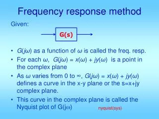
Why is Frequency Response Important? • Signals are easily represented in terms of sinusoidal functions • LTI systems are easily characterized in terms of frequency response • LTI systems are easily tested and verified using sinusoidal test signals • Relationship to Laplace transform and its rich framework • ∞ • G(jω)= G(s) │ =∫ f(t) e – jωtdt • s = j ω0 • Y(j ω) = G(jω)/[1 + G(jω) H(jω)] • ∞ • Y(j ω) ↔ y(t) = 1/2π ∫ F(jω) e jωt dω • - ∞ • Allows us to characterize steady-state response of LTI systems for design • Amplitude • Phase • Bandwidth • Assessing stability in the frequency domain • Gain Margin • Phase Margin • Nyquist Criterion
Why is Frequency Response Important? • Signals are easily represented in terms of sinusoidal functions • LTI systems are easily characterized in terms of frequency response • LTI systems are easily tested and verified using sinusoidal test signals • Relationship to Laplace transform and its rich framework • ∞ • G(jω)= G(s) │ =∫ f(t) e – jωtdt • s = j ω0 • Y(j ω)/R(jω) =G(jω)/[1 + G(jω) H(jω)] • ∞ • Y(j ω) ↔ y(t) = 1/2π ∫ F(jω) e jωt dω • - ∞ • Allows us to characterize steady-state response of LTI systems for design • Amplitude • Phase • Bandwidth • Assessing stability in the frequency domain • Gain Margin • Phase Margin • Nyquist Criterion
Why is Frequency Response Important? • Signals are easily represented in terms of sinusoidal functions • LTI systems are easily characterized in terms of frequency response • LTI systems are easily tested and verified using sinusoidal test signals • Relationship to Laplace transform and its rich framework • ∞ • G(jω)= G(s) │ =∫ f(t) e – jωtdt • s = j ω- ∞ • Y(j ω) = G(jω)/[1 + G(jω) H(jω)] • ∞ • Y(j ω) ↔ y(t) = 1/2π ∫ F(jω) e jωt dω • - ∞ • Allows us to characterize steady-state response of LTI systems for design • Amplitude • Phase • Bandwidth • Assessing stability in the frequency domain • Gain Margin • Phase Margin • Nyquist Criterion
G(jω) = G(s)│ = R(ω)+ j Xω) where R(ω) = Re{G(j ω) } and X(ω) = Im{G(j ω) } s = j ω Alternatively, G(jω) =│G(jω)│e jФ(ω) = │G(jω)│Ф(ω) Relationships: Ф(ω) = tan -1{X(ω) / R(ω) } and │G(jω)│2 = │R(ω)│2 + │X(ω)│2 Polar Plots
G(jω) = G(s)│ = R(ω)+ j Xω) where R(ω) = Re{G(j ω) } and X(ω) = Im{G(j ω) } s = j ω Alternatively, G(jω) =│G(jω)│e jФ(ω) = │G(jω)│Ф(ω) Relationships: Ф(ω) = tan -1{X(ω) /R(ω)} and │G(jω)│2 = │R(ω)│2 + │X(ω)│2 Polar Plots
G(jω) = G(s)│ = R(ω)+ j Xω) where R(ω) = Re{G(j ω) } and X(ω) = Im{G(j ω) } s = j ω Alternatively, G(jω) =│G(jω)│e jФ(ω) = │G(jω)│Ф(ω) Relationships: Ф(ω) = tan -1{X(ω) / R(ω) } and │G(jω)│2 = │R(ω)│2 + │X(ω)│2 Polar Plots
Polar Plot Example 1 G(s) = V2(s)/ V1(s) = 1/(RCs + 1) G(jω) = V2(jω)/ V1(jω) = 1/[RC jω + 1] = 1/[(jω/ω1)+ 1] where ω1 = 1/RC G(jω) =R(ω) + jX(ω) G(jω) = 1 – j(ω/ω1) /[1 + (ω/ω1)]2 G(jω) = {1 /[1 + (ω/ω1)]2} – j{(ω/ω1) /[1 + (ω/ω1)]2 } G(jω) =│G(jω)│ Ф(ω) │G(jω) │ = 1 /[1 + (ω/ω1) 2] 1/2 Ф(ω) = – tan -1(ω/ω1)
Polar Plot Example 1 G(s) = V2(s)/ V1(s) = 1/(RCs + 1) G(jω) = V2(jω)/ V1(jω) = 1/[RC jω + 1] = 1/[(jω/ω1)+ 1] where ω1 = 1/RC G(jω) =R(ω) + jX(ω) G(jω) = 1 – j(ω/ω1) /[1 + (ω/ω1)]2 G(jω) = {1 /[1 + (ω/ω1)]2} – j{(ω/ω1) /[1 + (ω/ω1)]2 } G(jω) =│G(jω)│ Ф(ω) │G(jω) │ = 1 /[1 + (ω/ω1) 2] 1/2 Ф(ω) = – tan -1(ω/ω1)
Polar Plot Example 1 G(s) = V2(s)/ V1(s) = 1/(RCs + 1) G(jω) = V2(jω)/ V1(jω) = 1/[RC jω + 1] = 1/[(jω/ω1)+ 1] where ω1 = 1/RC G(jω) =R(ω) + jX(ω) G(jω) = 1 – j(ω/ω1) /[1 + (ω/ω1)]2 G(jω) = {1 /[1 + (ω/ω1)]2} – j{(ω/ω1) /[1 + (ω/ω1)]2 } G(jω) =│G(jω)│ Ф(ω) │G(jω) │ = 1 /[1 + (ω/ω1) 2] 1/2 Ф(ω) = – tan -1(ω/ω1)
Polar Plot Example 1 G(s) = V2(s)/ V1(s) = 1/(RCs + 1) G(jω) = V2(jω)/ V1(jω) = 1/[RC jω + 1] = 1/[(jω/ω1)+ 1] where ω1 = 1/RC G(jω) =R(ω) + jX(ω) G(jω) = 1 – j(ω/ω1) /[1 + (ω/ω1)]2 G(jω) = {1 /[1 + (ω/ω1)]2} – j{(ω/ω1) /[1 + (ω/ω1)]2 } G(jω) =│G(jω)│ Ф(ω) │G(jω) │ = 1 /[1 + (ω/ω1) 2] 1/2 Ф(ω) = – tan -1(ω/ω1)
Polar Plot Example 2 G(s) │ = G(jω) = K/ jω(jωτ + 1) = K/ (jω – ω2 τ) s = jω │G(jω) │ = K/[ω 2+ ω4 τ 2) 1/2 Ф(ω) = – tan -1{1/ (–ω τ) } G(jω) =K/jω – ω2 τ) G(jω) = K(– j ω– ω2 τ)/(ω 2+ ω4 τ 2) R(ω) = – Kω2 τ /(ω 2+ ω4 τ 2) X(ω) = – Kω/(ω 2+ ω4 τ 2)
Polar Plot Example 2 G(s) │ = G(jω) = K/ jω(jωτ + 1) = K/ (jω – ω2 τ) s = jω │G(jω) │ = K/[ω 2+ ω4 τ 2) 1/2 Ф(ω) = – tan -1{1/ (–ω τ) } G(jω) =K/jω – ω2 τ) G(jω) = K(– j ω– ω2 τ)/(ω 2+ ω4 τ 2) R(ω) = – Kω2 τ /(ω 2+ ω4 τ 2) X(ω) = – Kω/(ω 2+ ω4 τ 2)
Polar Plot Example 2 G(s) │ = G(jω) = K/ jω(jωτ + 1) = K/ (jω – ω2 τ) s = jω │G(jω) │ = K/[ω 2+ ω4 τ 2) 1/2 Ф(ω) = – tan -1{1/ (–ω τ) } G(jω) =K/jω – ω2 τ) G(jω) = K(– j ω– ω2 τ)/(ω 2+ ω4 τ 2) R(ω) = – Kω2 τ /(ω 2+ ω4 τ 2) X(ω) = – Kω/(ω 2+ ω4 τ 2)
Polar Plot Example 2 G(s) │ = G(jω) = K/ jω(jωτ + 1) = K/ (jω – ω2 τ) s = jω │G(jω) │ = K/[ω 2+ ω4 τ 2) 1/2 Ф(ω) = – tan -1{1/ (–ω τ) } G(jω) =K/jω – ω2 τ) G(jω) = K(– j ω– ω2 τ)/(ω 2+ ω4 τ 2) R(ω) = – Kω2 τ /(ω 2+ ω4 τ 2) X(ω) = – Kω/(ω 2+ ω4 τ 2)
Polar Plot Example 2 G(s) = (K/ τ)/s(s + 1/τ) When s = jω G(jω) = (K/ τ)/ jω(jω + p) │G(jω1) │ = (K/ τ)/ │jω1││(jω1 + p) │ Ф(ω 1) = –(j ω1) – (j ω1 + p) Ф(ω 1) = –90 º –tan -1(ω1/p)
Polar Plot Example 2 G(s) = (K/ τ)/s(s + 1/τ) When s = jω G(jω) = (K/ τ)/ jω(jω + p) │G(jω1) │ = (K/ τ)/ │jω1││(jω1 + p) │ Ф(ω 1) = –(j ω1) – (j ω1 + p) Ф(ω 1) = –90 º – tan -1(ω1/p)
Polar Plot Example 2 G(s) = (K/ τ)/s(s + 1/τ) When s = jω G(jω) = (K/ τ)/ jω(jω + p) │G(jω1) │ = (K/ τ)/ │jω1││(jω1 + p) │ Ф(ω 1) = –(j ω1) – (j ω1 + p) Ф(ω 1) = –90 º – tan -1(ω1/p)