Frequency response method
This guide explores the frequency response method using G(jω) as a function of ω, defining the Nyquist plot and the amplitude and phase response. It explains the process of obtaining frequency response data both analytically by evaluating G(jω) and experimentally by measuring output in response to input signals. Key concepts such as system type, steady-state analysis, and the interpretation of Bode plots are covered. It provides examples of different system types and their corresponding frequency response characteristics, aiding in the design and analysis of control systems.

Frequency response method
E N D
Presentation Transcript
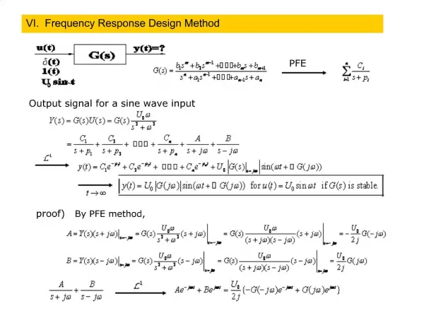
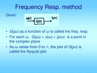
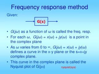
Frequency response method Given: • G(jω) as a function of ω is called the freq. resp. • For each ω, G(jω) = x(ω) + jy(ω) is a point in the complex plane • As ω varies from 0 to ∞, G(jω) = x(ω) + jy(ω) defines a curve in the x-y plane or the s=x+jy complex plane. • This curve in the complex plane is called the Nyquist plot of G(jw) G(s) nyquist(sys)
Can rewrite in Polar Form: • |G(jω)| as a function of ω is called the amplitude resp. • as a function of ω is called the phase resp. • The two plots: with log scale-ω, are Bode plot bode(sys)
To obtain freq. Resp from G(s): • Select • Evaluate G(jω) at those to get • Plot Imag(G) vs Real(G): Nyquist • or plot with log scale ω
To obtain freq. resp. experimentally: • Select • Give input to system as: • Adjust A1 so that the output is not saturated or distorted. • Measure amp B1 and phase φ1 ofoutput: System
Then is the freq. resp. of the system at freq ω1 • Repeat for all ωK • Either plot or plot
G1(s) G2(s) Product of T.F.
System type & Bode plot C(s) Gp(s)
System type is for steady state,i.e. t →∞ i.e. s → 0 i.e. ω → 0 As ω → 0 i.e. slope = N(–20) dB/dec.
N = 0, type zero: at low freq: mag. is flat at 20 log K phase plot is flat at 0°
If Bode gain plot is flat at low freq, system is type zero (confirm by phase plot flat at 0°) Then: Kv = 0, Ka = 0 Kp = Bode gain as ω→0 = DC gain (convert dB to values)
N = 1, type = 1 Bode mag. plot has –20 dB/dec at low freq. (ω→0) (straight line with slope = –20) Bode phase plot becomes flat at –90° when ω→0 Kp= DC gain → ∞ Kv = K = value of asymptotic straight line at ω = 1 =ws0dB =asymptotic straight line 0 dB crossing frequency Ka = 0
The matching phase plot at lowfreq. must be → –90° type = 1 Kp= ∞ ← position error const. Kv = value of low freq. straight line at ω = 1 = 23 dB ≈ 14 ← velocity error const. Ka = 0 ← acc. error const.
N = 2, type = 2 Bode gain plot has –40 dB/dec slope at low freq. Bode phase plot becomes flat at –180° at low freq. Kp= DC gain → ∞ Kv = ∞ also Ka = value of straight line at ω = 1 = ws0dB^2
Example Ka Sqrt(Ka)