Chapter 8 Frequency-Domain Analysis
Chapter 8 Frequency-Domain Analysis. Automatic Control Systems, 9 th Edition F. Golnaraghi & B. C. Kuo. 1, p. 409. 8-1 Introduction. For a LTI system: input -- steady-state output -- Sinusoidal steady-state analysis :. s = j . M ( s ). 1, p. 410. Frequency Response.

Chapter 8 Frequency-Domain Analysis
E N D
Presentation Transcript
Chapter 8Frequency-DomainAnalysis Automatic Control Systems, 9th Edition F. Golnaraghi & B. C. Kuo
1, p. 409 8-1 Introduction • For a LTI system: input -- steady-state output -- • Sinusoidal steady-state analysis: s = j M(s)
1, p. 410 Frequency Response • Closed-loop transfer function: • Sinusoidal steady-state transfer function: s = j Magnitude of M(j): Phase of M(j):
1, p. 411 Gain-Phase Characteristics cut-off frequency
1, p. 412 Frequency-Domain Specifications • Resonant Peak Mr:the maximum value of the relative stability of a stable closed-loop system • Resonant Frequency r:the frequency at which thepeak resonant Mr occurs • Bandwidth BW:the frequency at whichdrops to 70.7% of, or 3 db down from, its zero-freq. value the transient response properties of a control system • Cutoff Rate:the slope of at high frequency
2, p. 413 8-2 Mr, r, and Bandwidth of the Prototype Second-Order System • The prototype second-order system: • u = /n:magnitude: phase:
2, p. 414 Resonant Frequency and Resonant Peak • Resonant frequency r: • Resonant peak : Resonant frequency: r = 0 if 0.707 Mr = 1 if 0.707
2, p. 415 Magnification vs Normalized Frequency u = /n = 0 r = n
2, p. 416 Mr, urvs Damping Ratio
2, p. 417 Bandwidth • Definition: 70.7% or 3 dB
2, p. 417 Time-Domain Response vsFrequency-Domain Characteristics • Mr depends on only.The maximum overshoot also depends only on . • For 0.707, Mr = 1 and r = 0.The maximum overshoot is 0 when 1.0. • BW is directly proportional to n andinversely proportional to .The rise time tr increases as n decreases.BW and tr are inversely proportional to each other. • BW and Mr are proportional to each other for 0 0.707.
2, p. 419 Correlation between Pole Locations
2, p. 419 Unit-Step and Frequency Responses
3, p. 418 8-3 Effects of Adding a Zero to the Forward-Path Transfer Function zero: s = 1/T • closed-loop transfer function: • Bandwidth: increase BW
3, p. 421 Magnification Curves
3, p. 423 Unit-Step Responses: adding a zero
4, p. 424 8-4 Effects of Adding a Pole to the Forward-Path Transfer Function pole: s = 1/T Effects:Decrease BW,Increase Mr,Make the closed-loop system less stable
4, p. 425 Unit-Step Responses: adding a poles T tr BW Mr yrmax
5, p. 426 8-5 Nyquist Stability Criterion: Fundaments • The Nyquist plot of the loop transfer functionG(s)H(s), or L(s), is done in polar coordinates as varies from 0 to . • The Nyquist criterion has the following features: • In addition to providing the absolute stability, the Nyquist criterion also gives information on the relative stability of a stable system and the degree of instability of an unstable system. • The Nyquist plot is very easy to obtain. • The Nyquist plot gives information on the frequency-domain characteristics such as Mr, r, and BW. • The Nyquist plot is useful for systems with pure time delay.
5, p. 427 Stability Problem • Closed-loop transfer function: • Characteristic equation: • Stability conditions: • Open-loop stability: if the poles of the loop transfer function L(s) are all in the left-half s-plane. • Closed-loop stability: if the poles of the closed-loop transfer function or the zeros of 1+L(s) are all in the left-half s-plane.
5, p. 428 Encircled • A point or region in a complex function plane is said to be encircled by a closed path if it is found inside the path Point B is not encircled by the closed path . Point A is encircled by in the counterclockwise (CCW) direction.
5, p. 428 Enclosed • A point or region is said to be enclosed by a closed path if it is encircled in the CCW direction or the point or region lies to the left of the path when the path is traversed in the prescribed direction.
5, p. 429 Number of Encirclements and Enclosures • When a point is encircled by a closed path ,N = the number of times it is encircled. • N is positivefor CCW encirclement and negative for CW encirclement. B is encircled twicein the CCW direction A is encircled once or 2 radians by in the CW direction B is encircled twice or 4 radians by in the CW direction A is encircled oncein the CCW direction
5, p. 429 Locus in the (s)-plane • Suppose that a continuous closed paths is arbitrarily chosen in the s-plane, as shown in Fig. 8-17(a). • If s does not go through any poles of (s), then the trajectory mapped by (s) into (s)-plane is also a closed one, as shown in Fig. 8-17(b). single-valued mapping (s): single-valued function
5, p. 430 Principles of the Argument • Let (s) be a single-valued function that has a finite number of poles in the s-plane. • Suppose that an arbitrarily closed paths is chosen in the s-plane so that the path does NOT go through any one of the poles or zeros of (s). • The corresponding locus mapped in the (s)-plane will encircle the originas many times asthe difference between the number of zeros and poles of (s) that are encircled by the s-plane locus s. N = Z PN = number of encirclements of the origin made by the locus .Z = number of zeros of (s) encircled by the s-plane locus s.P = number of poles of (s) encircled by the s-plane locus s.
5, p. 431 Examples of Determination of N • N > 0 (Z>P): the (s)-plane locus will encircle the origin N times in the same direction as that of s. • N = 0 (Z=P): the (s)-plane locus will not encircle the origin of the (s)-plane. • N < 0 (Z<P): the (s)-plane locus will encircle the origin N times in the opposite direction as that of s.
5, p. 432 Illustrative Example The net angle traversed by the (s)-plane:
5, p. 433 Table 8-1
5, p. 434 Nyquist Path • The Nyquist path is definedto encircled the entireright-half s-plane. • The Nyquist path must notpass through any poles andzeros of (s).
5, p. 434 Nyquist Criterion (1/2) • (s) = 1 + L(s), L(s): loop transfer function the origin of the (s)-plane corresponds to the (1, j0) point in the L(s)-plane. • Steps of the application of Nyquist criterion to the stability problem: 1. The Nyquist path s is defined in the s-plane, as shown in Fig. 8-20. 2. The L(s) plot corresponding to the Nyquist path is constructed in the L(s)-plane. 3. The value of N, the number of encirclement of the (1, j0) point made by L(s) plot, is obsered. 4. The Nyquist criterion follows from Eq. (8-42),
5, p. 435 Nyquist Criterion (2/2) • Stability requirements:For closed-loop stability, Z must equal zero.For open-loop stability, P must equal zero. • The condition of stability according to Nyquist Criterion:for a closed-loop system to be stable, the L(s) plot must encircle the (1, j0) point as many times as the number of poles of L(s) that are in the right-half s-plane, and the encirclement, if any, must be made in the clockwise dircetion (if s is defined in the CCW sense).
6, p. 435 8-6 Nyquist Criterion for Systems with Minimum-Phase Transfer Functions Minimum-phase transfer function: • A minimum-phase transfer function does not have poles or zeros in the right-half s-plane or on the j-axis, excluding the origin. • For a minimum-phase transfer function L(s) with m zeros and n poles, excluding the poles at s = 0, when s = j and as varies from to 0, the total phase variation of L(j) is (nm)/2 radians. • The value of a minimum-phase transfer cannot become zero or infinity at any nonzero finite frequency. • A nonminimum-phase transfer function will always have a more positive phase shift as varies from to 0. Or equally true, it will always have a more negative phase as varies from 0 to .
6, p. 436 Nyquist Criterion for Systems with Minimum-Phase Transfer Functions • L(s): minimum-phase type P = 0Nyquist criterion N = 0 • For a closed-loop system with loop transfer function L(s) that is of minimum-phase type, • the system is closed-loop stable if the plot of L(s) that corresponds to the Nyquist path does NOT encircle (or enclose) the critical point (1, j0) in the L(s) -plane. • If the (1, j0) point is enclosed by the Nyquist plot, the system is unstable.
6, p. 437 Not Strictly Proper Transfer Function • The characteristic equation of a system:K: a variable parameterLeq: the equivalent transfer function • If Leq does not have more poles than zeros, • Plot the Nyquist-plot of 1/Leq(s)the critical point is still (1, j0) for K > 0the variable parameter on the Nyquist plot is now 1/K. the Nyquist criterion can still be applied
7, p. 437 8-7 Relation between the Root Loci and the Nyquist Plot • Both the root locus and the Nyquist criterion deal with the location of the roots of the characteristic equation of a linear SISO system. • Characteristic equation: • The Nyquist plot of L(s) in the L(s)-plane is the mapping of the Nyquist path in the s-plane. • The root locus must satisfyThe root loci simply represent a mapping of the real axis of L(s)-plane or the G(s)H(s)-plane onto the s-plane.
7, p. 438 Mapping s-plane onto G(s)H(s)-plane
7, p. 438 Mapping G(s)H(s)-plane onto s-plane
7, p. 439 Relation between G(s)H(s)- and s-planes
7, p. 439 Relation between G(s)H(s)- and s-planes
8, p. 440 8-8 Illustrative Examples: Nyquist Criterion for Min.-Phase Transfer Func. • Example 8-8-1: minimum-phase type Sketch of the Nyquist plot of L(j)/K 1. Substitute s = j in L(s): 2. Get the zero-frequency( = 0) property: 3. Get the infinite-frequency( = ) property:
8, p. 441 Example 8-8-1 (cont.) 4. Find the possible intersects on the real axis:Set the imaginary part of L(j)/K to zero:The intersect on the real axis of the L(j)-plane at ( must be positive)
8, p. 441 Example 8-8-1 (cont.) The intersect on the real axis of the L(j)-plane at • K<240: the intersect wouldbe to the rightof (1, j0).The critical point is notenclosed stable. • K=240: the intersect is atthe 1 point. marginally stable. • K>240: the intersect would be to the leftof (1, j0). unstable. • K<0: the critical point (+1, j0) is enclosed unstable.
8, p. 442 Example 8-8-1 (cont.) Stable: 0 < K < 240
8, p. 442 Example 8-8-2 Characteristic equation: Sketch the Nyquist plot of Leq(s): 1. 2. Two end points: 3. The possible intersects on the real axis: = 0 and Four imaginary roots
8, p. 443 Example 8-8-2 (cont.) Stable: K > 0
8, p. 444 Example 8-8-2 (cont.) Stable: K > 0
9, p. 444 8-9 Effects of Adding Poles and Zeros toL(s) on the Shape of the Nyquist Plot • Addition of Poles at s = 0: • Properties of Nyquist plot: multiplicity = p:
9, p. 445 Nyquist Plots Add a poleat s = 0 to L(s)
9, p. 446 Example 8-9-1
9, p. 447 Example 8-9-1 (cont.)