Chapter 4: Frequency Domain Processing

1. IUST Chapter 4:Frequency Domain Processing Image Transformations

2. Contents • Fourier Transform and DFT • Walsh Transform • Hadamard Transform • Walsh-Hadamard Transform (WHT) • Discrete Cosine Transform (DCT) • Haar Transform • Slant Transform • Comparison of various Transforms

3. Introduction • Although we discuss other transforms in some detail in this chapter, we emphasize the Fourier transform because of its wide range of applications in image processing problems.

4. Fourier Transform (1-D)

5. Fourier Transform (2-D)

6. Discrete Fourier Transform In the two-variable case the discrete Fourier transform pair is

7. Discrete Fourier Transform When images are sampled in a squared array, i.e. M=N, we can write

8. Discrete Fourier Transform Examples At all of these examples, the Fourier spectrum is shifted from top left corner to the center of the frequency square.

9. Discrete Fourier Transform Examples At all of these examples, the Fourier spectrum is shifted from top left corner to the center of the frequency square.

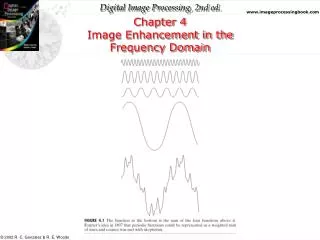
10. Discrete Fourier Transform Display At all of these examples, the Fourier spectrum is shifted from top left corner to the center of the frequency square.

11. Discrete Fourier Transform Example Main Image (Gray Level) DFT of Main image (Fourier spectrum) Logarithmic scaled of the Fourier spectrum

12. Discrete Fourier Transform MATLAB program page 1 from 3. • % Program written in Matlab for computing FFT of a given gray color image. • % Clear the memory. • clear; • % Getting the name and extension of the image file from the user. • name=input('Please write the name and address of the image : ','s'); • % Reading the image file into variable 'a'. • a=imread(name); • % Computing the size of image. Assuming that image is squared. • N=length(a); • % Computing DFT of the image file by using fast Fourier algorithm. • F=fft2(double(a))/N;

13. Discrete Fourier Transform MATLAB program page 2 from 3. • % Shifting the Fourier spectrum to the center of the frequency square. • for i=1:N/2; for j=1:N/2 • G(i+N/2,j+N/2)=F(i,j); • end;end • for i=N/2+1:N; for j=1:N/2 • G(i-N/2,j+N/2)=F(i,j); • end;end • for i=1:N/2; for j=N/2+1:N • G(i+N/2,j-N/2)=F(i,j); • end;end • for i=N/2+1:N; for j=N/2+1:N • G(i-N/2,j-N/2)=F(i,j); • end;end

14. Discrete Fourier Transform MATLAB program page 3 from 3. • % Computing and scaling the logarithmic Fourier spectrum. • H=log(1+abs(G)); • for i=1:N • H(i,:)=H(i,:)*255/abs(max(H(i,:))); • end • % Changing the color map to gray scale (8 bits). • colormap(gray(255)); • % Showing the main image and its Fourier spectrum. • subplot(2,2,1),image(a),title('Main image'); • subplot(2,2,2),image(abs(G)),title('Fourier spectrum'); • subplot(2,2,3),image(H),title('Logarithmic scaled Fourier spectrum');

15. Discrete Fourier Transform(Properties) • Separability The discrete Fourier transform pair can be expressed in the seperable forms:

16. Discrete Fourier Transform(Properties) • Translation The translation properties of the Fourier transform pair are :

17. Discrete Fourier Transform(Properties) • Periodicity The discrete Fourier transform and its inverse are periodic with period N; that is, F(u,v)=F(u+N,v)=F(u,v+N)=F(u+N,v+N) If f(x,y) is real, the Fourier transform also exhibits conjugate symmetry: F(u,v)=F*(-u,-v) Or, more interestingly: |F(u,v)|=|F(-u,-v)|

18. Discrete Fourier Transform(Properties) • Rotation If we introduce the polar coordinates Then we can write: In other words, rotating F(u,v) rotates f(x,y) by the same angle.

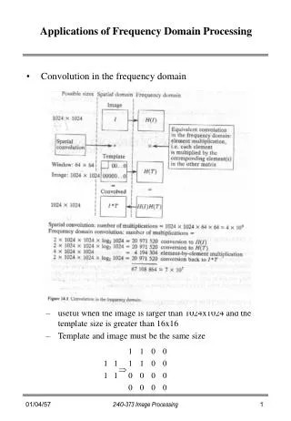
19. Discrete Fourier Transform(Properties) • Convolution The convolution theorem in two dimensions is expressed by the relations : Note :

20. Discrete Fourier Transform(Properties) • Correlation The correlation of two continuous functions f(x) and g(x) is defined by the relation So we can write:

21. Discrete Fourier Transform (Properties) • Sampling 1-D The Fourier transform and the convolution theorem provide the tools for a deeper analytic study of sampling problem. In particular, we want to look at the question of how many samples should be taken so that no information is lost in the sampling process. Expressed differently, the problem is one of the establishing the sampling conditions under which a continuous image can be recovered fully from a set of sampled values. We begin the analysis with the 1-D case. As a result, a function which is band-limited in frequency domain must extend from negative infinity to positive infinity in time domain (or x domain).

22. Discrete Fourier Transform (Properties) • Sampling 1-D f(x) : a given function F(u): Fourier Transform of f(x) which is band-limited s(x) : sampling function S(u): Fourier Transform of s(x) G(u): window for recovery of the main function F(u) and f(x). Recovered f(x) from sampled data

23. Discrete Fourier Transform (Properties) • Sampling 1-D f(x) : a given function F(u): Fourier Transform of f(x) which is band-limited s(x) : sampling function S(u): Fourier Transform of s(x) h(x): window for making f(x) finited in time. H(u): Fourier Transform of h(x)

24. Discrete Fourier Transform (Properties) • Sampling 1-D s(x)*f(x) (convolution function) is periodic, with period 1/Δu. If N samples of f(x) and F(u) are taken and the spacings between samples are selected so that a period in each domain is covered by N uniformly spaced samples, then NΔx=X in the x domain and NΔu=1/Δx in the frequency domain.

25. Discrete Fourier Transform (Properties) • Sampling 2-D The sampling process for 2-D functions can be formulated mathematically by making use of the 2-D impulse function δ(x,y), which is defined as A 2-D sampling function is consisted of a train of impulses separated Δx units in the x direction and Δy units in the y direction as shown in the figure.

26. Discrete Fourier Transform (Properties) • Sampling 2-D If f(x,y) is band limited (that is, its Fourier transform vanishes outside some finite region R) the result of covolving S(u,v) and F(u,v) might look like the case in the case shown in the figure. The function shown is periodic in two dimensions. (u,v) inside one of the rectangles enclosing R elsewhere The inverse Fourier transform of G(u,v)[S(u,v)*F(u,v)] yields f(x,y).

27. The Fast Fourier Transform (FFT) Algorithm

28. Other Seperable Image Transforms For 2-D square arrays the forward and inverse transforms are g(x,y,u,v) : forward transformation kernel h(x,y,u,v) : inverse transformation kernel The forward kernel is said to be seperable if g(x,y,u,v)=g1(x,u)g2(y,v) In addition, the kernel is symmetric if g1 is functionally equal to g2. In this case we can write: g(x,y,u,v)=g1(x,u)g1(y,v)

29. Other Seperable Image Transforms If the kernel g(x,y,u,v) is seperable and symmetric, also may be expressed in matrix form: Where F is the N×N image matrix, A is an N×N symmetric transformation matrix T is the resulting N×N transform. And for inverse transform we have:

30. Walsh Transform When N=2n, the 2-D forward and inverse Walsh kernels are given by the relations Where bk(z) is the kth bit in the binary representation of z. So the forward and inverse Walsh transforms are equal in form; that is:

31. Walsh Transform 1-D kernel In 1-D case we have : In the following table N=8 so n=3 (23=8). “+” denotes for +1 and “-” denotes for -1.

32. Walsh Transform This figure shows the basis functions (kernels) as a function of u and v (excluding the 1/N constant term) for computing the Walsh transform when N=4. Each block corresponds to varying x and y form 0 to 3 (that is, 0 to N-1), while keeping u and v fixed at the values corresponding to that block. Thus each block consists of an array of 4×4 binary elements (White means “+1” and Black means “-1”). To use these basis functions to compute the Walsh transform of an image of size 4×4 simply requires obtaining W(0,0) by multiplying the image array point-by-point with the 4×4 basis block corresponding to u=0 and v=0, adding the results, and dividing by 4, and continue for other values of u and v.

33. Walsh Transform Example Main Image (Gray Level) WT of Main image (Walsh spectrum) Logarithmic scaled of the Walsh spectrum

34. Walsh Transform (WT) MATLAB program page 1 from 3. • % Program written in Matlab for computing WT of a given gray color image. • clear; • % Getting the name and extension of the image file from the user. • name=input('Please write the name and address of the image : ','s'); • a=imread(name); • N=length(a); • % Computing Walsh Transform of the image file. • n=log2(N);n=1+fix(n);f=ones(N,N); • for x=1:N; for u=1:N • p=dec2bin(x-1,n); q=dec2bin(u-1,n); • for i=1:n; f(x,u)=f(x,u)*((-1)^(p(n+1-i)*q(i))); • end;end;end • F=(1/N)*f*double(a)*f;

35. Walsh Transform (WT) MATLAB program page 2 from 3. • % Shifting the Fourier spectrum to the center of the frequency square. • for i=1:N/2; for j=1:N/2 • G(i+N/2,j+N/2)=F(i,j); • end;end • for i=N/2+1:N; for j=1:N/2 • G(i-N/2,j+N/2)=F(i,j); • end;end • for i=1:N/2; for j=N/2+1:N • G(i+N/2,j-N/2)=F(i,j); • end;end • for i=N/2+1:N; for j=N/2+1:N • G(i-N/2,j-N/2)=F(i,j); • end;end

36. Walsh Transform (WT) MATLAB program page 3 from 3. • % Computing and scaling the logarithmic Walsh spectrum. • H=log(1+abs(G)); • for i=1:N • H(i,:)=H(i,:)*255/abs(max(H(i,:))); • end • % Changing the color map to gray scale (8 bits). • colormap(gray(255)); • % Showing the main image and its Walsh spectrum. • subplot(2,2,1),image(a),title('Main image'); • subplot(2,2,2),image(abs(G)),title('Walsh spectrum'); • subplot(2,2,3),image(H),title('Logarithmic scaled Walsh spectrum');

37. Hadamard Transform When N=2n, the 2-D forward and inverse Hadamard kernels are given by the relations Where bk(z) is the kth bit in the binary representation of z. So the forward and inverse Hadamard transforms are equal in form; that is:

38. Hadamard Transform 1-D kernel In 1-D case we have : In the following table N=8 so n=3 (23=8). “+” denotes for +1 and “-” denotes for -1.

39. Hadamard Transform This figure shows the basis functions (kernels) as a function of u and v (excluding the 1/N constant term) for computing the Hadamard transform when N=4. Each block corresponds to varying x and y form 0 to 3 (that is, 0 to N-1), while keeping u and v fixed at the values corresponding to that block. Thus each block consists of an array of 4×4 binary elements (White means “+1” and Black means “-1”) like Walsh transform. If we compare these two transforms we can see that they only differ in the sense that the functions in Hadamard transform are ordered in increasing sequency and thus are more “natural” to interpret.

40. Hadamard Transform Example Main Image (Gray Level) HT of Main image (Hadamard spectrum) Logarithmic scaled of the Hadamard spectrum

41. Hadamard Transform (HT) MATLAB program page 1 from 3. • % Program written in Matlab for computing HT of a given gray color image. • clear; • % Getting the name and extension of the image file from the user. • name=input('Please write the name and address of the image : ','s'); • a=imread(name); • N=length(a); • % Computing Hadamard Transform of the image file. • n=log2(N);n=1+fix(n);f=ones(N,N); • for x=1:N; for u=1:N • p=dec2bin(x-1,n); q=dec2bin(u-1,n); • for i=1:n; f(x,u)=f(x,u)*((-1)^(p(n+1-i)*q(n+1-i))); • end;end;end • F=(1/N)*f*double(a)*f;

42. Hadamard Transform (HT) MATLAB program page 2 from 3. • % Shifting the Fourier spectrum to the center of the frequency square. • for i=1:N/2; for j=1:N/2 • G(i+N/2,j+N/2)=F(i,j); • end;end • for i=N/2+1:N; for j=1:N/2 • G(i-N/2,j+N/2)=F(i,j); • end;end • for i=1:N/2; for j=N/2+1:N • G(i+N/2,j-N/2)=F(i,j); • end;end • for i=N/2+1:N; for j=N/2+1:N • G(i-N/2,j-N/2)=F(i,j); • end;end

43. Hadamard Transform (HT) MATLAB program page 3 from 3. • % Computing and scaling the logarithmic Hadamard spectrum. • H=log(1+abs(G)); • for i=1:N • H(i,:)=H(i,:)*255/abs(max(H(i,:))); • end • % Changing the color map to gray scale (8 bits). • colormap(gray(255)); • % Showing the main image and its Hadamard spectrum. • subplot(2,2,1),image(a),title('Main image'); • subplot(2,2,2),image(abs(G)),title('Hadamard spectrum'); • subplot(2,2,3),image(H),title('Logarithmic scaled Hadamard spectrum');

44. Walsh-Hadamard Transform (WHT)

45. 1-D WHT Kernel Functions

46. 2-D WHT Kernel Functions

47. WHT and Fourier Transform

48. WHT Example

49. Discrete Cosine Transform

50. Discrete Cosine Transform (DCT) Each block consists of 4×4 elements, corresponding to x and y varying from 0 to 3. The highest value is shown in white. Other values are shown in grays, with darker meaning smaller.