Making Measurements
Making Measurements. Precision vs Accuracy. Accuracy : A measure of how close a measurement comes to the actual, accepted or true value of whatever is measured. Example : Over two trials, a student measures the boiling point of ethanol and then calculates the average.

Making Measurements
E N D
Presentation Transcript
Precision vs Accuracy • Accuracy : A measure of how close a measurement comes to the actual, accepted or true value of whatever is measured. • Example: Over two trials, a student measures the boiling point of ethanol and then calculates the average. Accepted Value = 78.4°C • She then checks a chemistry handbook (CRC) to see how close her measurements are to the actual value.
Precision vs Accuracy • Precision : A measure of how close a series of measurements are to one another. This is best determined by the deviation of the data points. • Example: Two students independently determine the average boiling point of ethanol. Accepted Value = 78.4°C • Student A’s data is less accurate but more precise than student B’s.
׀ error ׀ X 100 Accepted value ׀ 79.0-78.4 ׀ %E = X 100 78.4 Determining Error • Error : The difference between the accepted value and the experimental value. Formula: Error = experimental value – accepted value • Percent error : The absolute value of the error divided by the accepted value, multiplied by 100. Formula: % Error = • Calculate the % error for the data given below. Student A = 79.0 °C Accepted Value = 78.4 °C %E = 0.8 %
Scientific Notation • Scientific Notation : An expression of numbers in the form m x 10n where m is ≥ 1 and < 10 and n is an integer.. • Using scientific notation makes it easier to work with numbers that are very large and very small. • Example #1: A single gram of hydrogen contains approximately 602 000 000 000 000 000 000 000 atoms which can be rewritten in scientific notation as 6.02 x 10²³ • Example#2: The mass of an atom of gold is 0.000 000 000 000 000 000 000 327 gram which can be rewritten in scientific notation as 3.27 x 10⁻²²
Coefficient Exponent Scientific Notation • In scientific notation, there is a coefficient and an exponent, or power. 6.02 x 10²³ • The exponent value is determined by moving a decimal point. • For example: When changing a large number to scientific notation, the decimal is moved left until one non-zero digit remains. 6 02 atoms 000 000 000 000 000 000 000
Scientific Notation • Remember to count the number of place values as you move the decimal. 6 02 000 000 000 000 000 000 000 atoms 23 places • Now drop the “trailing” zeros and add an “x 10”.
Scientific Notation • Remember to count the number of place values as you move the decimal. 6 02 x 10 atoms 23 places • Now drop the “trailing” zeros and add an “x 10”. • Place the 23 as an exponent of the “10”. • You have just converted standard notation to scientific notation 6.02 x 10²³ 602 000 000 000 000 000 000 000
Scientific Notation • When changing a very small number to scientific notation, the decimal is moved to the right until it passes a non-zero number. 0 000 000 000 000 000 000 000 3 27 gram - 22 places • Again, count the number of place values the decimal moved.
Scientific Notation • When changing a very small number to scientific notation, the decimal is moved to the right until it passes a non-zero number. 0 000 000 000 000 000 000 000 3 27 gram - 22 places • Again, count the number of place values the decimal moved. • Now drop the “leading” zeros and add an “x 10”.
3 27 Scientific Notation • When changing a very small number to scientific notation, the decimal is moved to the right until it passes a non-zero number. x 10 gram - 22 places • Again, count the number of place values the decimal moved. • Now drop the “leading” zeros and add an “x 10”.
3 27 Scientific Notation • When changing a very small number to scientific notation, the decimal is moved to the right until it passes a non-zero number. x 10 gram - 22 • Again, count the number of place values the decimal moved. • Now drop the “leading” zeros and add an “x 10”. • Finally, place the -22 as an exponent of the “10”. • Again you have converted standard notation to scientific notation 3.27 x 10⁻²² 0.000 000 000 000 000 000 000 327
Scientific Notation • Normally, scientific notation is not used for measurements that produce an exponent of +1 or -1. Examples : 89.1 = 8.91 x 101 (not usually done) 0.32 = 3.2 x 10⁻¹ (not usually done) Practice problems • Change the following number to proper scientific notation. 0.000 000 12 = 1.2 x 10⁻⁷ • Change the following number to proper standard notation. 4.3 x 105 = 430 000
°C 25 24 23 22 Smallest division Recording Measurements • Assume you are using a thermometer and want to record a temperature. To do this, you must first determine the instrument’s precision, or I.P. The precision of an instrument is equal to the smallest division on the instrument’s scale. • Pictured to the right is a thermometer scale. What is the scale’s precision? The I.P. is = 0.1 °C
°C 25 24 23 22 Recording Measurements • The next thing to do is record the temperature and unit. How would you record the temperature shown? • If you recorded the temperature as 24.3 °C then you were not being as precise as you could be with the scale given. • If you look carefully at the top of the thermometer’s fluid you will see it rises a bit higher than 24.3 °C. You might now record the temperature as 24.31 °C or 24.32 °C
°C 25 24 23 22 Estimated digit Certain or known digits Significant digits Recording Measurements • The first three digits in our measurements are known with certainty. However, the last digit was estimated and involves some uncertainty. 24.32 °C • All measurements consist of known digits and one estimated digit. Together, they are called significant digits.
°C 25 24 23 22 Tolerance interval Significant figures Unit Recording Measurements • Error in measurement may be represented by a tolerance interval. • Machines used in manufacturing often set tolerance intervals, or ranges in which product measurements will be tolerated before they are considered flawed. • To determine the tolerance interval in a measurement, add and subtract (±) one-half of the precision of the measuring instrument to the measurement. • We will now express our measurement as 24.32 °C ± 0.05 °C (±T.I.)
°C 76 75 74 73 72 71 to match the place value of the T.I. This 3rd digit was rounded down 70 Recording Measurements • Always round the experimental measurement or result to the same decimal place as the uncertainty. It would be confusing (and perhaps dishonest) to suggest that you knew the digit in the hundredths (or thousandths) place when you admit that you’re unsure of the tenth’s place. • For example: How would you read the temperature shown to the right? It should be read as… 73.2 °C ± 0.1 °C (±T.I.)
Recording Measurements • Note: It is not necessary to write the tolerance interval for each measurement of a series of measurements made using the same instrument. Accepted value = 27.74 °C • For example: If you record a series of temperature measurements in a data table, then you need only state the tolerance interval once. • Keep in mind there are many ways of showing uncertainty in measurement. This is why you must indicate the source of the uncertainty, such as… Tolerance Interval (T.I.) Standard deviation (± SD) Standard error (± SE) Percent error (%E)
√ Zeros that do nothing but set the decimal point are not significant. √ Trailing zeros that aren’t needed to hold a decimal point are significant. Determining Significant Figures • Significant figures are all the digits that can be known precisely in a measurement, plus a last estimated digit. • The rules for recognizing significant figures are as follows: √Zeros within a number are always significant. Both 4308 and 40.05 contain four sig. figs. 570 000 and 0.010 and 310 contain two sig. figs. Both 4.00 and 0.0320 contain three sig. figs.
Determining Significant Figures • Here is a “trick” that can help you with significant figures. • Question: How many sig. figs. are in 0.00180 ? Step 1: Check to see if the number has a decimal. If yes, think “present.” If no, think “absent.” In our example of 0.00180, a decimal is present. Step 2: Note that Present starts with a “P” and so does Pacific. Pacific Ocean (decimal present)
Step 4: Draw an arrow from the Pacific Ocean through the number until you encounter a non-zero digit. Determining Significant Figures Step 3: Now place the number inside the U.S.A. pictured below. √ Rule: All digits to the right of the arrow tip are significant. In our example, 0.00180 has three significant figures. Pacific Ocean (decimal present) 0.00180
Determining Significant Figures • New Question: How many sig. figs. are in 403 200? Step 1: Check to see if the number has a decimal. If yes, think “present.” If no, think “absent.” In our example of 403 200, a decimal is absent. Step 2: Note that Absent starts with an “A” and so does Atlantic. Pacific Ocean (decimal present) Atlantic Ocean (decimal absent)
Step 4: Draw an arrow from the Atlantic Ocean through the number until you encounter a non-zero digit. Determining Significant Figures Step 3: Now place the number inside the U.S.A. pictured below. √ Rule: All digits to the left of the arrow tip are significant. In our example, 403 200 has four significant figures. Pacific Ocean (decimal present) Atlantic Ocean (decimal absent) 403 200
Determining Significant Figures • How many sig. figs are in each of the following measurements? five 280.00 five 2.8000 x 10 2 two 4.5 x 10 2 two 450 one 0.0003 two 0.00030 three 2.00 x 10 -4 seven 100.0030
mm 149 150 200 Determining Significant Figures • Let’s apply what you have learned. How would you record the following measurement? It should have been recorded as 150.00 mm ± 0.05 mm • Now change this measurement into scientific notation. It should have been written as 1.5000 x 10 2± 0.05 mm • Note that the three zeros after the numeral 5 must be retained in order to uphold the precision of the measurement. • How many significant figures does 1.5000 x 10² contain? It contains five.
Calculating with Significant Figures • In general, a calculated answer cannot be more precise than the least precise measurement from which it is calculated. This is analogous to saying that a chain cannot be stronger than its weakest link. • Here is the rule for Adding or Subtracting significant figures Round the answer to the same number of decimal places (not digits) as the measurement with the least number of decimal places. • Here is the rule for Multiplying or Dividing significant figures Round the answer to the same number of significant figures as the measurement with the least number of significant figures.
The first measurement (349.0 meters) has the least number of digits (one) to the right of the decimal point. Calculating with Significant Figures • Example addition problem: 12.52 + + 8.24 349.0 Step 1: Stack the numbers and align them by decimal location 369.76 369.76 Step 2: Add the numbers Step 3: Locate the measurement with the least number of digits to the right of the decimal point Step 4:The answer must be rounded to one digit after the decimal point. 369.8 or 3.698 x 10²
Calculating with Significant Figures • Example multiplication problem: 0.70 m x 2.10 m Step 1: Multiply the numbers 1.47 m2 1.47 m2 The first measurement (0.70) has smallest number of significant figures (two). Step 2: Locate the measurement with the least number of significant figures. Step 3: The answer must be rounded to the same number of significant figures as the measurement with the least number of significant figures 1.5 m2
10th’s place 5.2 x 10⁻² + 0.182 x 10⁻² Evaluate 5.2 x 10⁻² + 1.82 x 10⁻³ Change to same exponents 5.4 x 10⁻² 7.0 x 10⁵ - 0.52 x 10⁵ Evaluate 7.0 x 10⁵ - 5.2 x 10⁴ Change to same exponents 10th’s place Calculating with Scientific Notation • Example addition problem in scientific notation 5.382 x 10⁻² • Example subtraction problem in scientific notation 10th’s place 6.48 x 10⁵ 6.5 x 10⁵
Evaluate 2 x 10 -3 x 3.6 x 10 4 Round to 1 sig. fig. Evaluate 1.2 x 10 7 Round to 2 sig. figs. 4.7 x 10 2 Calculating with Scientific Notation • Example multiplication problem in scientific notation Multiply the coefficients Add the exponents 7 x 10 1 x 10 1 7.2 • Example division problem in scientific notation Divide the coefficients Subtract the exponents x 10 5 = 0.255319148 2.6 x 10 4
Calculating with Significant Figures Calculator answer Rounded answer Scientific notation Problem (2 sf) 2.4 x 10² 240 236.0869565 5.43 0.023 5 x 101 (1 sf) 47.2 236 x 0.2 50 (1 p) 9.25 x 10³ 9250.3 0.300 + 9 250 9250 (0.1 p) 2.268 x 10² 226.84 236.04 - 9.2 226.8 (1 p) 6.70 x 10 4 - 3.6 x 10 -2* 6.7 x 104 66999.964 67000 (2 sf) 2.04 x 10 -3x 1.2 x 10 2 2.4 x 10⁻¹ 0.24 0.2448 * Change to 67000 x 100 – 0.036 x 100