Download
1 / 34
340 likes | 536 Vues
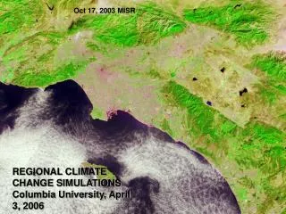
Oct 17, 2003 MISR. REGIONAL CLIMATE CHANGE SIMULATIONS Columbia University, April 3, 2006.

E N D
Oct 17, 2003 MISR REGIONAL CLIMATE CHANGE SIMULATIONS Columbia University, April 3, 2006
One-way nested modeling has been applied to climate change studies in the last few years. This technique consists of using output from GCM simulations to provide initial and driving lateral meteorological boundary conditions for high-resolution regional climate model simulations, generally with no feedback from the regional climate model to the driving GCM. Hence, a regional increase in resolution can be attained through the use of nested regional climate models to account for sub-GCM grid-scale forcings. This is attractive because regional models can introduce sensitivities at the landscape scale to the simulation. Moreover, as climate change impacts on ecosystems, air pollution, water resources etc. take place on the comparable scales, they may provide more relevant information to models of other earth system components.
Experimental Design model: MM5 boundary conditions: eta model reanalysis resolution: domain 1, 54 km, domain 2, 18 km, domain 3, 6 km time period: 1995 to present. One can think of this as a reconstruction of weather conditions over this time period consistent with three constraints: (1) our best guess of the large-scale conditions, (2) the physics of the MM5 model, and (3) the prescribed topography, consistent with model resolution.
VALIDATION This shows the correlation of daily-mean wind speed and direction between model and observations at 18 locations. Both wind speed and direction are reasonably well-correlated at all locations, in spite of many possible reasons for disagreement, including systematic and random measurement error. This gives confidence that the timing and magnitude of circulation anomalies are correct in the simulation.
WATER VAPOR FEEDBACK Water vapor feedback is thought to be a positive feedback mechanism. Water vapor feedback might amplify the climate’s equilibrium response to increasing greenhouse gases by as much as a factor of two. It acts globally. Increase in temperature Increase in water vapor in the atmosphere Enhancement of the greenhouse effect
SURFACE ALBEDO FEEDBACK Surface albedo feedback is thought to be a positive feedback mechanism. Its effect is strongest in mid to high latitudes, where there is significant coverage of snow and sea ice. Increase in temperature Increase in incoming sunshine Decrease in sea ice and snow cover
Equilibrium response of a climate model when feedbacks are removed.
To understand how cloud feedback might work, you have to understand some facts about clouds: (1) Clouds absorb radiation in the infrared, and therefore have a greenhouse effect on the climate. If you put a cloud high in the atmosphere, it will have a stronger greenhouse effect than if you put it low in the atmosphere. (2) Clouds reflect sunshine back to space. So more clouds means less sunshine for earth. If you put a cloud high in the atmosphere, it will reflect about the same amount of sunshine as if you put a cloud low in the atmosphere.
Reduced greenhouse effect Which effect is stronger depends on the geographical and vertical distribution of the decrease in cloudiness Decrease in cloudiness? Increased sunshine Models predict both an increase and decrease in cloudiness, and both positive and negative cloud feedbacks. Increase in temperature CLOUD FEEDBACK Enhanced greenhouse effect Which effect is stronger depends on the geographical and vertical distribution of the increase in cloudiness Increase in cloudiness? Reduced sunshine
Transient vs Equilibrium climate response Transient responserefers to the evolution of the climate system as it responds to external forcing, such as an increase in greenhouse gases. Equilibrium responserefers to the final state of the climate system after it has adjusted to the external forcing. The magnitude of the equilibrium response compared to the magnitude of the forcing is referred to as theclimate sensitivity.
Evolution of simulated global mean temperature when CO2 changes This shows the warming in a climate model when two scenarios of CO2 increases are imposed: one is a 1% per year increase in CO2 leading to a CO2 doubling, and the other is an increase at the same rate leading to a CO2 quadrupling. It shows that the warming continues for several centuries even when CO2 levels are stabilized, leading to significant differences between transient and equilibrium climate responses to external forcing.
The difference between the transient and equilibrium responses of a climate model to increasing greenhouse gases varies a great deal geographically.
The colors show 21st century warming taking place in response to a plausible scenario of radiative forcing. The values are averaged over all the ~20 simulations used in the most recent UN Intergovernmental Panel on Climate Change Report. The warming is calculated by subtracting temperatures at the end of the 20th century (1961-1990) from temperatures at the end of the 21st century (2071-2100).
The thin blue lines show the range in warming across all the models.
The thick green lines show the ratio of the mean change in temperature to the standard deviation of the temperature change.
HYDROLOGIC CYCLE INTENSIFICATION Increase in greenhouse gases means more longwave radiation reaches the surface Increase in evaporation (fairly uniform globally) Increase in precipitation (not uniform) Increase in temperatures favors loss of surface heat through evaporation rather than sensible heat
Colors show the simulated 21st century percent change in precipitation averaged over the simulations of the UN Intergovernmental Panel on Climate Change 3rd assessment report.
The red lines show the range in the percent increase in precipitation.
The thick green lines show the ratio of the mean change in precipitation to the standard deviation of the precipitation change.
Leung and Ghan (1999) imposed 2XCO2 conditions from CCM3 on a regional model based on MM5 covering the Pacific Northwest. They found the regional model has a different temperature sensitivity than the parent model, suggesting feedbacks operating on scales smaller than those resolved by the parent model are influencing sensitivity. They suggest this stems from the fact that in the parent model snow feedback processes are inadequately resolved in this region of intense topography.
The regional simulation shows a large reduction in snow cover at elevations near the present-day snow line (1000-2000 m). This is due to reduced snowfall and increased snow melt.
The Union of Concerned Scientists recently published an assessment of climate change in California. They based their assessment on the results from two global climate models, one with a relatively low sensitivity to CO2 doubling (PCM), and the other with a relatively high sensitivity (HADCM3). They looked at outcomes in California for two scenarios. One is “business as usual” scenario, that envisages fossil fuel emissions increasing at approximately the same rate as present for the remainder of the 21st century. The other is a lower emissions scenario, where emissions continue to increase but at a lower rate, stabilizing around 2050, then declining to levels below the present level by 2100. The global models’ resolutions are on the order of 200 km. Regional details have been supplied using a statistical downscaling technique.
Diminishing Sierra Snowpack% Remaining, Relative to 1961-1990 This shows how the more sensitive global model projects snowpack to change in the Sierras. The change in snowpack is significant because it comprises approximately half the total water storage capacity of California, the other half being contained mainly in human-made reservoirs. Source: A Luers/Union of Concerned Scientists
Most precipitation over the Sierras falls in wintertime, where it is stored in the snow pack. The snowpack comprises approximately half the total water storage capacity of California, the other half being contained mainly in human-made reservoirs.
As the snow melts, water flows to reservoirs, where it makes its way through aqueducts to agricultural and urban areas. This shows aqueducts for water resource re-distribution in California
The Sierra snow pack has been steadily shrinking over the past century… Sacramento River Runoff (1906-2001) April to July as a Percent of Total Runoff Source: California Protection Agency, Environmental Protection Indicators for California, 2001
The large-scale conditions in this regional simulation originated from transient climate-change simulations using the coupled ocean–atmosphere global climate model ECHAM4/OPYC (300-km grid). The regional details are supplied by a 50 km regional model (HIRAM). (Change = 2071-2100 minus 1961-1990) The relative change in the mean five-day precipitation for July–September that exceeds the 99th percentiles in scenario A2 with respect to the control Relative percentage change in precipitation for July–September in the Intergovernmental Panel on Climate Change's A2 scenario with respect to the present day Christensen & Christensen, Nature 2003
How credible are these results in light of this divergence in the global models?
CONCLUSIONS Like their global counterparts, predictions of regional climate change are most credible when they involve a plausible set of physical mechanisms. So far, the regional climate predictions that can be taken the most seriously involve temperature-cryosphere feedbacks. Regional climate predictions are subject to misinterpretation because their high resolution gives a false impression of fidelity. This is particularly true in the case of the predictions of local changes in the hydrologic cycle. There is huge divergence in hydrologic cycle intensification, and these signals are poorly understood in global models.