Lecture 5: source detection.

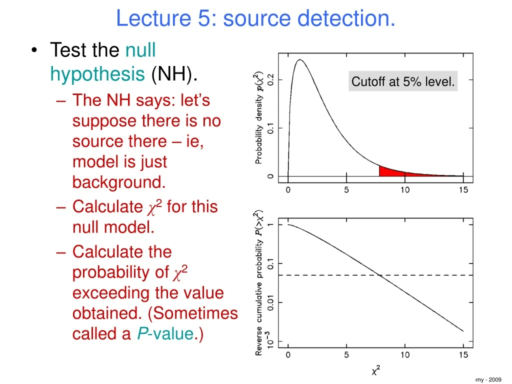
1. Lecture 5: source detection. • Test the null hypothesis (NH). • The NH says: let’s suppose there is no source there – ie, model is just background. • Calculate χ2 for this null model. • Calculate the probability of χ2 exceeding the value obtained. (Sometimes called a P-value.) Cutoff at 5% level.

2. Source detection. • If this probability (the P-value) is smaller than a previously chosen cutoff, call this a positive detection. • BUT! Note that there is no certainty. • Sometimes the null model will by chance give a large χ2 => ‘false positives.’ For given data, background and cutoff, there will be a fixed number of false positives expected in the source list. • => ‘reliability’. More on this later. • Sometimes a real source will give a small null-hypothesis χ2 => ‘false negatives’, real sources which are missed. • => ‘completeness’. More on this later.

3. Problems with the NH approach: • We don’t have exact knowledge of the background. • Have to estimate it either from • separate data – in which case we need separate data! • or from the same data… but this may be dominated by the source... • Or our background model may be wrong. • Same issues as other model fitting. In particular: • χ2 has to be used with care when the noise is Poisson.

4. But where are the sources? • A low probability for the null hypothesis tells us, at best, that there is a source somewhere. • Finding the source(s) consists rather of looking for peaks in a random signal. • The simplest example is when the noise is uncorrelated and the source peaks have width=0.

5. A generic source-detection algorithm • We shall assume that: • The data is ‘binned’ (eg CCD data). • We have a good independent estimate of the background. • The sources are sparsely distributed – such that we can deal with them one at a time. • The shape of the source profile is known. • The source position is unknown. • The source amplitude is unknown (but >0).

6. Generic source-detection algorithm: The algorithm has 3 steps: 1: Calculate a sliding-window map. 2: Find the peaks in this map. Choose a Pcutoff 3: For each peak, calculate the probability that it could arise by chance from the background (the null hypothesis P-value). P < Pcutoff? No Yes Sources Rejects

7. 1: The sliding window. y U y U y U

8. 1: The sliding window. • For each position of the sliding window, a single number U is calculated from the values falling within the window. • The output is a map of the U values. • The intent is to: • Raise the signal-to-noise • Improve sensitivity • Amplify the sources at the expense of the noise. • Sliding-window processing only has value when the source has a width > 1 pixel. • Edges need special treatment. Same thing.

9. 1: Window functions • A weighted sum (= a convolution). • Simplest with all weights = 1: “sliding box”. • Optimum weights – a “matched filter”: • For uniform Gaussian noise, wopt = s. • Trickier to optimize for Poisson noise. • Per-window null-hypothesis χ2. • With either an independent value of bkg (in which case degrees of freedom = number of pixels Nw in the window), or… • …one fitted from the data (deg free = Nw-1). • Likelihood (same bkg provisions as χ2).

10. 1: Window functions Parent function Data

11. 1: Window functions Parent function Chi squared, size=100 Matched filter, size=10 Log-likelihood, size=100

12. 2: Peak finding Gaussian noise, convolved with a gaussian filter. …don’t get the gaussians mixed up!

13. 2: Peak finding • No single neat prescription. • Naive prescription: • Pixel i is a peak pixel if yi > any other y within a patch of pixels from i-j to i+j. • But what value to choose for j? • Things to avoid are: • j too small – results in more than 1 peak per source; • j too large – misses a close adjacent source.

14. 2: Peak finding Box too small: Box too large:

15. 3: Decision time – is it a source or not? • To calculate a P-value we need the probability distribution of peaks in the post-window map of U values (given the null hypothesis). • This is not the same as the probability distribution of the original data values… • …nor is it even the same as the probability distribution of U values. • In fact, little work seems to have been done on ppeaks. (Though there is quite a lot on the distribution of extrema – not quite the same thing.)

16. 3: The decision ‘Map’ vs ‘peak’ distributions for Gaussian noise. Black: all pixels Red: peaks

17. 3: Cash to the rescue • First of all, remember that our model m has p parameters θ = [θ1, θ2,… θp]. • Cash theory – form a ratio between 2 likelihoods: • The numerator is calculated with all p parameters fixed at their ‘null hypothesis’ values. • For the denominator, a subset, q in number, of the parameters are adjusted to give the highest likelihood value. • -2log(this ratio) behaves like χ2 with q degrees of freedom.

18. 3: Cash to the rescue • A practical recipe for applying Cash to source detection goes as follows: • Choose a window area surrounding each peak. • Within this window, calculate Lnull with model mi = bi (the background map values). • Calculate Lbest by fitting a model • Degrees of freedom ν = 1 (the amplitude) + d (the dimensions of the spatial fit). • The Cash statistic 2(Lbest-Lnull) behaves like χ2 with 1+d deg. free. mi = bi + θ1s(ri – θr)

19. 3: Cash to the rescue • The only difficult point (which is a problem for every method) is to calculate the fraction of pixels which are peaks. • Monte Carlo • Possibly a Fourier technique? • Also, don’t want to use the fit for final parameter values. A Mighell fit is better.

20. Useful references: • W Press et al, “Numerical Recipes in Fortran” • P Bevington, “Data reduction and error analysis for the physical sciences” • W Cash, Ap J 228, 939 (1979) • K J Mighell, Ap J 518, 380 (1999) • I M Stewart, A&A 454, 997 (2006) • I M Stewart, A&A, in print (2009) • Wikipedia