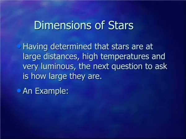
Dimensions of Stars

1. Dimensions of Stars • Having determined that stars are at large distances, high temperatures and very luminous, the next question to ask is how large they are. • An Example:

2. Dimensions of Stars • The star Betelgeuse (a Orionis) has the following parameters: • Distance 150 pc • Apparent magnitude 0 • Absolute magnitude -6 • Relative luminosity 104 L¤ • Temperature 3000 K (I.e., a class M star).

3. Dimensions of Stars • The luminosity depends on the surface area of the star (µR2) and T 4 (from Stefan’s law). • Hence, the ratio of the radii of Betelgeuse and the Sun is: • R / R¤ = (T¤ / T )2 (L / L¤)1/2 = 370 • This corresponds to almost 2 AU – I.e., larger than the orbit of Mars (1.5 AU)!

4. 106 1000 R¤ 100 R¤ Supergiants 104 10 R¤ 1 R¤ Main sequence 102 Giants 0.1 R¤ Luminosity (L¤) 1 Sun 0.01 R¤ 10-2 0.001 R¤ Red dwarfs White dwarfs 10-4 40,000 20,000 10,000 5,000 2,500 Temperature (K) Dimensions of Stars • Applying the same technique to other stars allows lines of constant radii to be plotted on the HR diagram.

5. Dimensions of Stars • Note: • Most stars on the main sequence have radii similar to the Sun, but that, as we have shown, the luminous red stars have large radii. • White dwarfs have very small radii – comparable to that of the Earth!

6. Luminosity and Spectral Class • Can the luminosity be deduced directly from the spectral class? • No - e.g. Betelgeuse and Barnard’s Star are both class M, but the latter is 18 stellar magnitudes fainter • Details of the spectrum provides a handle:

7. Luminosity and Spectral Class • Absorption line shapes: • Narrow lines Þ Low density, hence large dimensions • Broad lines Þ High density, hence a compact object Hg Rigel, a B8 supergiant Hd The B8 main sequence component of Algol

8. 106 I 104 II III 102 IV V 1 Luminosity (L¤) 10-2 10-4 2,500 20,000 5,000 10,000 40,000 Temperature (K) Luminosity and Spectral Class • Such studies lead to the idea of Luminosity Classes • Labelled I to V in order of decreasing luminosity • Provides another handle on distance • “Spectroscopic Parallax”

9. Spectroscopic Parallax • Example: • The star a Leonis (Regulus) has an apparent magnitude of 1.4 and its spectrum shows it to be a B7V star. • This gives an absolute magnitude of -0.6. • The distance modulus is therefore 2, giving a distance of 25 pc.

10. Spectroscopic Parallax • Note: • The luminosity classes are broad and poorly defined. Hence, a distance determined by this method should be regarded as an estimate • This method has nothing to do with Parallax!

11. Masses of Stars • We have now established methods of measuring : • Distance • Brightness • Composition • Temperature • Size

12. Masses of Stars • we require the mass to gain a complete picture of the properties of stars. • For example: • are giant and dwarf stars proportionatly more massive than the Sun, or are they about the same? • How does mass vary along the main sequence?

13. Masses of Stars • It is impractical to measure the mass of an isolated star. • Many stars occur in gravitationally bound multiple systems – in particular, binary stars. • By observing the orbits of such stars (and knowing the distance), the total mass can be found

14. a M1 M2 Masses of Stars • Application of Kepler’s Third Law • Miin Solar Masses, a in AU and P the orbital period in years

15. Masses of Stars • Example: • The orbit of the binary star 70 Ophiuchi (parallax 0.2 arc sec) has been plotted over many years. • The period is 87.7 years • The semi-major axis is 4.5 arc sec. • What is the sum of the masses of the two stars?

16. Masses of Stars • 70 Ophiuchi • Distance = 5pc • ~ 106 AU. • Hence, the semi-major axis is ~ 22 AU. • The period is 87.7 years • The total mass is ~ 1.4 M¤

17. a2 a1 M1 M2 Masses of Stars • The ratio of the masses: • The two stars orbit a common centre of mass • The major axes of the two ellipses are in the inverse ratio of the masses. M1/M2 = a2/a1

18. Masses of Stars • Together with the sum of the masses, the individual masses can now be obtained. • Orbital period Þ Total mass • Ratio of major axes Þ Ratio of masses

19. Masses of Stars • Binary systems containing red giants: • show masses of red giants fall into the same range as main sequence stars • confirming our conjecture they have low densities) • White dwarfs are found to have masses about 1 M¤ • indicating these are very dense objects!

20. Luminosity, L (Solar Luminosities) L = M 7/2 Mass, M (Solar Masses) Mass-Luminosity Relationship • Is there a relationship between luminosity and mass?

21. Mass-Luminosity Relationship • L = M7/2 • Approximate relationship • Valid for low mass stars up to about 1 solar mass • L = M3 gives better fit for high mass stars • Note for Main Sequence stars only

22. Stellar Interiors • Basic Ideas • Hydrostatic Equilibrium • Classical and Quantum Gases • Electron and photon gases • Ionisation • The Saha Equation • Heat Transfer Mechanisms • Fusion

23. Hydrostatic Equilibrium • Since main sequence stars are stable, and are neither expanding or contracting, they are clearly in equilibrium • Internal pressure supports against gravity

24. Hydrostatic Equilibrium • We wish to examine: • The relationship between mean pressure and potential and kinetic energies • The Virial Theorem • The consequences of equilibrium of non-relativistic and ultra-relativistic gases

25. Dr R g(r)DM (P+DP)DA P.DA r Mass DM Hydrostatic Equilibrium • Consider a volume element in a spherical system of mass M and radius R

26. Hydrostatic Equilibrium • Net force due to the pressure gradient • Noting that the mass, DM, of the element is: DM = r(r)Dr DA, and including the gravitational force, g(r) we have the acceleration of the volume element:

27. Hydrostatic Equilibrium • In equilibrium, net acceleration is zero. • Hence: • We can write g(r) as Where m(r) is the mass contained within a radius r

28. Hydrostatic Equilibrium • Therefore, if the star is to be in hydrostatic equilibrium, the pressure gradient at any distance r from the centre is:

29. = dm Hydrostatic Equilibrium • We can use this expression to relate the average pressure to the total gravitational potential • Multiply both sides by 4pr3 • Integrate from 0 to R

30. Hydrostatic Equilibrium • The right hand side is simply the gravitational potential: • The left hand side can be evaluated using integration by parts:

31. = 0 = dV = -3<P >V Hydrostatic Equilibrium • The left-hand side then becomes:

32. Hydrostatic Equilibrium • Hence, the average pressure in a system in hydrostatic equilibrium and with gravitational potential Egis: • The Virial Theorem

33. Hydrostatic Equilibrium • Non-relativistic (p << mc)vs. ultra-relativistic (p >> mc) gases. • Fundamental relationships:

34. Hydrostatic Equilibrium • Non-relativistic gases: • p.v. = mv2 • Hence: • Pressure = 2/3 kinetic energy density

35. Hydrostatic Equilibrium • Consequences: • Hence:

36. Hydrostatic Equilibrium • Since: • i.e., the system is bound with binding energy -Etotal = internal kinetic energy

37. Hydrostatic Equilibrium • Implications: • Tightly bound systems are hot • Energy loss from a gas cloud causes contraction and heating • 1/2 loss of gravitational energy goes into radiation, 1/2 into raising the temperature • Increase in temperature provides pressure to counter gravity • Excess energy production in a star causes expansion and cooling

38. Hydrostatic Equilibrium • Ultra-relativistic gases: • p.v. = pc • P >>mc, so EKE= pc • Hence: • Pressure = 1/3 kinetic energy density

39. Hydrostatic Equilibrium • Consequences: • EKE= -Eg • System only in equilibrium if Etotal = 0 • Hydrostatic equilibrium of ultra-relativistic particles (e.g., photon gas, high energy electron gas) easily disrupted.

40. Next Lecture: • Classical and Quantum Gases • The Saha Equation • Derivation • Consequences for ionisation and absorption