Download
1 / 60
600 likes | 776 Vues
Long-run trends in the concentration of income and wealth. Daniel Waldenström (IFN, Stockholm). Presentation at 3rd GLOBALEURONET Summer School, Paris School of Economics, July 10, 2008. THE ISSUES. What are the long-run cross-country trends in the concentration of income and wealth?

E N D
Long-run trends in the concentration of income and wealth Daniel Waldenström (IFN, Stockholm) Presentation at 3rd GLOBALEURONET Summer School, Paris School of Economics, July 10, 2008
THE ISSUES • What are the long-run cross-country trends in the concentration of income and wealth? • The role of industrialization? • The role of globalization? • Other determinants?
THIS TALK • Part I: Wealth • Long-run trends and revisit impact of industrialization • Sample: 7 countries (old and new data) • Time period: From mid-18th century to present day • Part II: Income • Long-run determinants of top income shares • Role of some economic variables • Sample: 16 countries • Time period: 1900-2000 • Conclusions & some unresolved issues
Part I: The long-run concentration of wealth: An overview of recent findings
Outline of Part I • Starting point • Wealth concepts and definitions • Country results: • France • Switzerland • UK • US • Denmark • Norway • Sweden • Cross-country comparison • Conclusions
1. Starting point Issues of interest: • Common vs. specific trends • Heterogeneity within the top • Did wealth inequality increase in the initial phase of industrialization? (Kuznets hypothesis) • Role of wars, taxes, globalization of the 20th century • The role of the Scandinavian Welfare State?
Starting point (2) • Historical data on wealth inequality: • France, 1807-1994 (Piketty et al, 2006) • Switzerland, 1913-1997 (Dell et al, 2005) • United Kingdom, 1740-2003 (several authors) • United States, 1774-2002 (several authors) • Denmark, 1789-1996 (various sources) • Norway, 1789-2002 (various sources) • Sweden, 1800-2006 (various sources) • Variation across these countries: • Timing of industrialization • Participation in World Wars • Level of wealth taxation
2. Wealth concepts and definitions • A mix of sources • Estate tax data • Wealth tax data • Survey data • Wealth concept • Net worth = real and financial assets less debts • Does (typically) not include: art & jewelry, TV:s etc, pension wealth, human capital, public goods • A mix of observational units • Households (wealth tax-based, survey sources) • Individuals (deceased, estate-tax based sources)
Concepts (cont’d) • Computation of top wealth shares: • Estimate share of total net worth that goes to the top 10, 5, 1, 0.1, etc % of all potential wealth holders. • Reference total wealth: All personal wealth (not only taxed wealth) estimated from tax records or national accounts • Reference total for the population: All potential tax units (not just those who file tax returns) • Problems with tax-based data • Evasion, avoidance etc. • Importance grows with systematic differences across distribution and over time • We lack compositional information (except for France)
U.K. wealth concentration, 1774-2001 Lindert (2000) Atkinson et al IRS (2006)
U.S. wealth concentration, 1774-2001 Lindert (2000) Shammas (1993) Kopzcuk & Saez (2004) Wolff (1987, ...)
Swedish wealth concentration, 1870-2006 Crises, Home ownership, Welfare State Globalization Industrialization Top 1% ? Top 10-1% Bottom 90%
What happened in Sweden after 1980? … and why does it not show up in the official statistics? • Unique Swedish combination of the 1980s & 90s: • High taxes on wealth, inheritance and capital income • Financial market boom • Liberalized capital account (after 1989) • Effect: Large fortunes ”disappear” • Private wealth (and its holders) leave Sweden • Capital in Sweden transfered to closely held companies What does this do to the distribution of wealth?
Swedish wealth concentration 1950-2005 (official series) Bottom 90% Wealth share (%) Top 1%
Swedish wealth concentration 1950-2005 (our new series) Bottom 90% Wealth share (%) Top 1%
How do we estimate the wealth of the rich? • We add fortunes to the wealth of the richest percentile in the domestic population Three additions: • Foreign household wealth • Net errors and omissions in the Balance of Payments • ”Unexplained savings” in the Financial Accounts • Family-firm wealth of rich Swedes in Sweden • Listings of super rich Swedes since 1983 • Wealth of rich Swedes abroad • Listings of super rich Swedes since 1983
Net errors and omissions (N.E.O.) Accumulated net errors and omissions over GDP
Net errors and omissions (N.E.O.) Accumulated net errors and omissions over GDP
Top 1% - Sweden’s official series Wealth share (%) SCB official
Effect by adding foreign household wealth Wealth share (%) + N.E.O. SCB official
Effect by adding family-firm wealth of rich Swedes living in Sweden + Rich in Sweden Wealth share (%) + N.E.O. SCB official
Effect by adding wealth of rich Swedes abroad + Rich abroad + Rich in Sweden Wealth share (%) + N.E.O. SCB official
Comparing Sweden and the U.S. (SCF) + Rich abroad + N.E.O, rich in USA and abroad USA + Rich in Sweden Wealth share (%) + N.E.O. SCB official
Summarizing Part I • Industrialization’s impact on wealth mixed • 20th century sees massive wealth equalization • Owner-occupied housing • Wars, crises and progressive taxation • Role of government mixed (public provision of shooling, health, pensions, increase inequality of net worth) • What about the Kuznets inverse-U theory? • No clear increase in inequality during industrialization, but a clear decrease thereafter • That is, rather an inverse-J curve... • International capital flows may imply that national wealth concentration is underestimated
Part II: The long-run determinants of inequality: What can we learn from top income data?
Starting point • New database on long-run income inequality: • Top income shares • General dissatisfaction with available inequality data • scattered • short time periods • different across countries making comparisons difficult • A solution: use tax data • available since the early 20th C. Long-run series • available in most countries cross-country comparisons • before WWII, primarily top incomes observed • focus on the rich important for analyzing driving factors
Income inequality data • Top income data: • Main concept: gross total income before taxes/transfers • Tax units: individuals or households • Composition: labor, capital, business income included • Realized capital gains not included* • Computation of top income shares: • Share of total income of the top 10, etc % of all potential income earners. • Reference income not only taxed income • Reference population not just those who file tax returns
France • Piketty, 2003, Journal of Political Economy
United States • Piketty and Saez, 2003, Quarterly J of Econ.
Sweden • Roine and Waldenström, 2008, J of Public Ec.
Other countries... • Canada (Saez and Veall, 2005, AER) • United kingdom (Atkinson, 2005, J Roy Stat Soc) • Switzerland & Germany (Dell, 2005, JEEA) • Netherlands (Atkinson and Salverda 2005, JEEA) • Australia (Atkinson and Leigh, 2006) • New Zealand (Atkinson and Leigh, 2006, RevIncWealth) • India (Banerjee and Piketty, 2005, WBER) • Japan (Moriguchi and Saez, 2006, ReStat) • Finland (Riihilä et al, 2005) • Spain (Alvaredo and Saez, 2006) • Argentina (Alvaredo, 2006) • Ireland (Nolan, 2007) • China (Piketty and Qian, 2006) • Indonesia (Leigh and van der Eng, 2006) • Norway (Aaberge and Atkinson, 2008) • Underway: Portugal, Denmark, South Africa, African colonies New OUP volumes edited by Atkinson & Piketty
Main findings in top income literature • Long-run top income trends strikingly similar • Up to 1980, income inequality decreases • After 1980, some divergence seem to arise • Anglo-Saxon countries experience surge in top shares • Continental European countries remain on low levels • Differences within the top: • Top precentile has large share of capital income • Rest of top decile mainly highly paid wage earners • Suggested causes (based on country cases): • Shocks to capital reduces before WWII • Progressive taxation holds back increase after WWII • After 1980: many candidates...
This analysis • Use new panel with long-term top income shares • Divide the income distribution into three groups: • The Rich (Top 1 percentile) • The Upper Middle Class (Top10–1 percentiles) • The Rest (Bottom 90 percentiles) • Try to relate their income shares to other variables: • Economic growth, Trade openness, Financial development, Growth of government • Allow effects to differ between • Levels of economic development (low/medium/high) • Anglo-Saxon countries and ”rest of the world” • Bank-oriented vs market-oriented financial systems
Potential determinants of inequality • Economic growth • Top incomes are more closely tied to the economy (bonuses, incentive contracts) • Trade openness • Standard: Capitalists gain in capital abundant countries • ”Superstars” in global labor markets (Rosen, 1980; Gersbach & Schmutzler, 2007) • Financial development • Typically seen as pro-poor • Reduces credit constraints, pools resources (Beck et al. 2007) • When is finance pro-rich? • When the rich have control over politics and finance • At early stages of development (Greenwood & Jovanovic 1990)
Potential determinants of inequality • Marginal income taxation • Two potential effects from higher top marginal tax: • Lowers pre-tax income through reduced incentives to work • Raises pre-tax income to compensate for tax increase Altogether: Theory provides conflicting answers
Data (cont’d) • Other variables: • GDP/capita and Population • Source: Maddison • Financial development: Bank deposits + Stock market • Sources: Mitchell, IFS, FSD, Bordo, Rajan & Zingales • Trade openness: (Exports+Imports)/GDP • Sources: Mitchell, López-Córdoba & Meissner, Bordo • Central government spending • Sources: Mitchell, Rousseau & Sylla, Bordo, IFS, FSD • Top marginal tax rates • Sources: Top inc studies, OECD, Rydqvist et al., Bach et al,
First look at the data • Several common chocks clearly visible • Great depression • WWII • Effects from globalization can be common to the countries in our sample • This makes them hard to trace statistically
Variable plots GDP/cap Total capitalization Gov. spending Openness
Variable plots Marginal tax rate (Preferred) (rate at inc= 5xGDP/cap, statutory) Marginal tax rate 2 (statutory)
Econometric method • We model top income shares as being function of: • financial development, trade openness, government spending, tax progressivity, economic growth • Obviously, we cannot claim to establish causality. • We use five-year period averages in analysis • The panel dataset is long and narrow • Fixed effects model (de-meaning) not optimal • Measurement errors likely to be serially correlated Use first-differenced model (Bound & Krueger, 1991)