Download
1 / 43
430 likes | 448 Vues
This paper discusses the importance of rescheduling in production schedules and proposes various rescheduling methods and strategies. It also introduces the PISCES system for controlling expedition and scheduling in logistics.

E N D
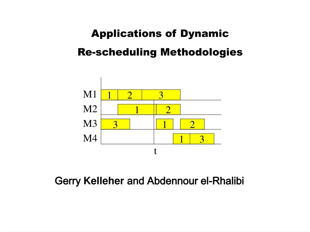
M1 1 2 3 M2 1 2 M3 3 1 2 M4 1 3 Applications of Dynamic Re-scheduling Methodologies t Gerry Kelleher and Abdennour el-Rhalibi
Introduction Preparing predictive schedule is not enough. there are many events that require the revision of the predictive schedule. a frequent comment in many scheduling contexts is that scheduling is not a problem but rescheduling is
Terminology Rescheduling, process of updating an existing production schedule in response to disruptions Disruptions (Rescheduling Factors) • Machine Failure • Urgent Job Arrival • Job cancellation • Due date change • Operator Absenteeism • Change in Job Priority • Delay in Arrival • Rework or Quality Problems • Over or under estimation of processing times
Terminology Scheduling, creating production schedules and Rescheduling framework, consists of rescheduling environment, rescheduling strategies, rescheduling policy and rescheduling methods
Triggering Events The current schedule has become infeasible The current schedule is likely to fail based on some performance measures Detection of opportunities to improve the schedule while the current schedule is still acceptable Rescheduling is done with fixed frequency
Rescheduling Framework Rescheduling Strategies (any environment with variability) Dynamic (no schedule) Predictive-reactive (generate and update) Dispatching rules Control-theoretic Rescheduling Policies) Periodic Event-driven Hybrid Rescheduling Methods (for predictive-reactive) Schedule Generation Schedule Repair Nominal Schedules Robust Schedules Right-shift Rescheduling Partial Rescheduling Complete Regeneration
Rescheduling Strategies Dynamic Scheduling do not use scheduling policies, uses current information to dispatch the jobs (eg FIFO, EDD, SPT…) tradeoff utility, measure of improvement, against stability, measure of nervousness three types of actions upon information arrival: no move, repair and reschedule.
Dynamic Scheduling Utility, a measure of improvement such as, decrease in total completion time • Stability, a measure of nervousness, such as, total change in start times and completion times • Utility & Stability vs. time of arrival information and/or change in the current system • Decide on repair or reschedule
Predictive-Reactive Scheduling Evaluation step, generate a robust schedule, evaluating the impact that a disruption causes Solution step, determine rescheduling solutions enhancing the current performance Revision step, update the existing schedule or generate a new one
Rescheduling Methods Right shift rescheduling, postpones each remaining operations Partial rescheduling, schedules only operations affected by the disruption • Matchup scheduling, reschedule all the jobs before a matchup point • If point too large, use integer programming or dispatching rules Regeneration, reschedule the entire jobs before the rescheduling point
P I S C E S (Pipeline Intermodal System to Support Control Expedition and Scheduling) IN-96-SC.1204 Partners: Fraser Williams Logistics Ltd. Van Ommeren Agencies Rotterdam BV Liverpool John Moores University PROJECT FUNDED BY THE EUROPEAN COMMISSION UNDER THE TRANSPORT RTD PROGRAMME OF THE 4TH FRAMEWORK PROGRAMME
PISCES and Logistics Evolution Total Integration 2000s Fragmentation 1960s Evolving Integration 1980s Demand Forecasting Purchasing Warehousing Requirements Planning Production Planning Materials Management Manufacturing Inventory Warehousing Logistics Materials Handling Industrial Packaging PISCES Physical Distribution • Inventory Distribution Planning Transportation Order Processing Transportation Customer Service
Global carrier Manufacturer Distribution Centre Transportation Pipeline Intermodal System to Support Control Expedition and Scheduling Freight Forwarder Bookings Cargo receipts Packing lists Shipping advice Cargo Manifests Shipment Status Pre advice of container contents PISCES Database Customs documentation Customs clearance Check commodity availability/location Accept shipments into inventory PO Delivery Details Wholesaler/Retailer
EQUIPMENT SERVICES/ EVENTS INFORMATION Pipeline Intermodal System to Support Control Expedition and Scheduling VELOCITY CRITICAL PATH • Speed of information transfer related to need • Neutral database to maintain relationships • No need to publicise actual parties or cargo details • Integrate info/services/equipment to flex critical path • Provide adaptive algorithms for scheduling/optimisation • Focus on ‘operational’ milestones • Easy access via Internet
Support to Logistics Management Decisions Location Choice Transport Mode Selection Vendor Choice STRATEGIC Uncertainty Time frame Throughput levels Employment levels Distribution routes TACTICAL Scope Vehicle scheduling Order tracking Inventory replenishment OPERATIONAL
ContainerTransport Delivery Empty Running Delivery DEPOT CUSTOMER Delivery Collection Positioning Delivery PORT Collection CUSTOMER Delivery DEPOT Collection Positioning CUSTOMER
ContainerTransport Delivery Empty Running Delivery DEPOT CUSTOMER Delivery 3 Positioning 4 Empty Collection PORT 1 Delivery CUSTOMER Collection Delivery 2 DEPOT 6 5 Collection Positioning Collection CUSTOMER
Rotterdam Amsterdam Antwerp Hannover Cologne Trier Duisberg Bonn Dortmund Metz Munich Strasbourg Stuttgart Basel Transport Scheduling
Rotterdam Amsterdam Antwerp Hannover Cologne Trier Duisberg Bonn Dortmund Metz Munich Strasbourg Stuttgart Basel Transport Scheduling
Transport Scheduling Constraints on Length/Durationof Tour Time Window Pickup andDelivery CONTAINERS TRANSPORT TRIANGULATION: CONSTRAINTS DynamicChanges Multiple Types of Vehicles Multiple Ports/Depots Capacited Vehicles Containers/GoodsCompatibility Intermodality
Transport Scheduling Total Traveled Distance Empty Running Cost SCHEDULING OptimisationCriteria RESCHEDULING Maximise Length of Triangulated Legs Maximise Use of Intermodal Alternative:Barge/Train Minimise Changes from the Initial Routing Minimise Delays Minimise Introduction of New Resources
Design of a Software Package to Produce Routing Scheduler Application to the Triangulation Problem, for the Transport of Containers. Application to Classical Vehicle Routing Problems. • We take advantage of two techniques by using an hybrid approach: • a CSP program to compute feasible solutions on a subspace of the search space. • a GA to explore the space formed by the solutions provided by the CSP, and perform the optimisation
CONSIGNMENT DATABASE MANAGEMENT PROGRAMS Routing Scheduler Reasoning Module Optimisation Module Selection CSP Solver Feasible solutions Parent Infeasible solutions Recombination Mutation CSP Generator Variables Domains Constraints Population Repaired solutions Offspring Forward Checking/ Orderings Replacement Constraint Satisfaction and Genetic Algorithm
Performance on Van Ommeren’s Problems Triangulation of Containers Transport
Tyre Manufacturing (Pirelli) • Problem - add rescheduling capability to an existing system - BIS (Banbury Information System • Scheduling of the Banbury Area is a job-shop scheduling task input to the system is a production plan containing customers and production orders (denoted requirements – typically ~50 per day). • Scheduling horizon varies with the due-date of the orders, ( typically ~2 days).
Scheduling difficult, complex in itself but also requires reaction in real-time to change: • small revisions because of short stops of machines. • major revisions because of breakdown • customer order changes • feedback from quality control on finished tyres • breakdowns in semi-manufacturing, building and curing areas.
The objectives to be optimised include: 1. Minimise the tardiness of the requirements 2. Keep stock-levels within a defined minimum/maximum 3. Optimise the standing times of compounds 4. Maximise machine utilisation 5. Minimise set-up-time for the machines 6. Use prioritised machines
Cause Typical frequency (times/week) Typical Duration (hours) Banbury breakdown 1 - 2 2 - 8 Banbury stoppages < 1 1 - 24 Rework ~ 3 Lack of raw-material sometimes Change in requirements seldom Table 1 Causes of Rescheduling
Shift1 Shift2 Shift3 Zone 1 Zone 2 Rescheduling Time DAY 1 DAY 2 Shift1 Shift2 Shift3 Reaction Time Dosage Time Dosage Horizon Zone 4 Zone 3 Time Zones for Rescheduling
Disruption Weight max Zone 4 Zone 1 Zone 3 Zone 2 time Disruption Function Weighting
Evaluation criteria BIS TRIS prototype TRIS final prototype Number of real time changes to schedule 2-3 per day 1-2 per day < 1 per day Number of re-scheduling Not available Not available 1-2 per week “Out of stock” (per day) < 1 per day < 1 per day < 1 per day Stock levels (total batches) 1300 -1450 1200 -1300 < 1000 Lateness 3-4 per day 1-2 per day < 1 per day Use of highest priority machine 93 % 93 % 94-95 % Machine saturation 90 % 94 % 93-97 % Lead time factor 80 % 90 % > 90 % WIP ~ 100 ~ 100 ~ 100 Standing time 1-4 hours 1-4 hours 1-4 hours Average set-up ~ 5 mins ~ 5 mins ~ 3-4 mins Preparation of data 2-3 hours 30-40 mins 30-40 mins Manual revision of the schedule 2 hours 2 hours 30 mins
Notes and Conclusion Cost of rescheduling policies depends on frequency of rescheduling Implementation of rescheduling policy depends on information acquisition More research on the interaction of rescheduling policies with other production planning decisions is needed
Size of Disruption This refers to the duration for which the schedule is subject to disruptions, such as machine breakdown. This expressed as a percentage of the initial’s schedule makespan. Incidence of the disruption This refers to the time of occurrence of the disruption, which can occur either early or late in the schedule. Size of the Schedule This refers to the size of the scheduling problem, and is expressed as the number of job operations present in the initial schedule. Schedule Structure This refers to the tightness of the schedule, as it shows in the Gantt chart. We can also estimate it by considering the difference of values the utility function (e.g. makespan) of the worst and best solution found by CSP/GA Rescheduling
Levels of experiment Disruption Dimension Problem Category (PC1) 1 Problem Category (PC2) 2 Size of disruption Machine Breakdown Small 1-5% of Makespan Large 6-10% of Makespan Process time Change Small 1-5% of Makespan Large 6-10% of Makespan Urgent Job Process Time about 1-5% of Makespan Process Time about 1-5% of Makespan Incidence of disruptions Early 5-55% of Makespan Late 60%-90% of Makespan Schedule size Small <200 operations (about 10 jobs) Large 200-300 operations (about 20 jobs) Schedule structure Tight (<100) / Loose(>100) Tight (<100) / Loose(>100)
Table 29: Classification JSSP Benchmarks Table 29: Classification JSSP Benchmarks Problem Instance name Size of Problems Size of Schedule Incidence of Disruptions Size of Disruptions orb1 10x10 PC1 Early (5-55%) Small (1%-5%) orb2 10x10 PC1 Late (60%-90) Large(6%-10%) orb3 10x10 PC1 Early (5-55%) Large(6%-10%) orb4 10x10 PC1 Late (60%-90) Small(1%-5%) orb5 10x10 PC1 Early (5-55%) Small(1%-5%) abz5 10x10 PC1 Late (60%-90) Large(6%-10%) abz6 10x10 PC1 Early (5-55%) Large(6%-10%) abz7 20x15 PC2 Late (60%-90) Small(1%-5%) ab8 20x15 PC2 Early (5-55%) Small(1%-5%) abz9 20x15 PC2 Late (60%-90) Large(6%-10%) la19 10x10 PC1 Early (5-55%) Large(6%-10%) la20 10x10 PC1 Late (60%-90) Small(1%-5%) la21 15x10 PC1 Early (5-55%) Small(1%-5%) la24 15x10 PC1 Late (60%-90) Large(6%-10%) la25 20x10 PC2 Early (5-55%) Large(6%-10%) la27 20x10 PC2 Late (60%-90) Small(1%-5%) la29 20x10 PC2 Early (5-55%) Small (1%-5%) la36 15x15 PC2 Late (60%-90) Large(6%-10%) la38 15x15 PC2 Early (5-55%) Large(6%-10%) la39 15x15 PC2 Late (60%-90) Small (1%-5%) la40 15x15 PC2 Early (5-55%) Small (1%-5%)
Efficiency defined as the percentage change in makespan of the repaired schedule compared to the preschedule where, h = Efficiency Mnew = Makespan of the rescheduled schedule Mo = Makespan of the preschedule
Stability is the absolute sum of difference in starting times of the job operations between the initial and the rescheduled schedules. It is then normalized as a ratio of total number of operations in the schedule. A schedule will be stable if it deviates minimally from the preschedule. where, x = Normalized deviation. pj = number of operations of job j. k = number of jobs. Sji* = Starting time of ith operation of job j in repairedschedule. Sji= Starting time of ith operation of job j in original schedule.
Table 31: Efficiency and Stability of rescheduling (machine breakdown) Problem Description RSR Efficiency % AOR Efficiency % CSP/GA Efficiency % RSR Stability % AOR Stability % CSP/GA Stability % orb1-10x10 PC1/ Early /Small/tight 96-97% 97-100 91-98% 8-11% 1-3% 1-4% orb2-10x10 PC1/Late / Large/loose 88-94% 95-96% 94-99% 4-9% 1-2% 1% orb3-10x10 PC1/Early/ Large/tight 84-89% 92-97% 97-98% 11-17% 4-9% 10-13% orb4-10x10 PC1/Late / Small/tight 95% 95-100% 98-99% 2-3% 1-2% 2% Orb5-10x10 PC1/Early / Small/tight 94-99% 100% 97-98% 7-9% 3 4-6% abz5-10x10 PC1/Late / Large/loose 92-93% 96-97% 93% 33-38% 17-25% 11-29% Abz6-10x10 PC1/Early / Large/loose 59-70% 72-79% 81-82% 43-68% 12-19% 26% abz7-20x15 PC2/Late/ Small/tight 94% 99% 96-97% 3-6% 1-2% 4% ab8- 20x15 PC2/Early Small/tight 91-93% 93-98% 91% 18-19% 9-13% 14% Abz9- 20x15 PC2/Late / Large/tight 83-92% 91-94% 87-98% 43-45% 21% 17-23%
Problem Description RSR Efficiency % AOR Efficiency % CSP/GA Efficiency % RSR Stability % AOR Stability % CSP/GA Stability % la19- 10x10 PC1/Early Large/loose 82-87% 86-93% 84-85% 71-75% 34-35% 24-37% la20-10x10 PC1/Late / Small/tight 92-97% 92-98% 93% 5-7% 2-3% 2-4% la21-15x10 PC1/Early / Small/tight 83-90% 96-98% 94-97% 10-14% 2-7% 5-9% la24-15x10 PC1/Late / Large/tight 88-89% 91-96% 95% 14-17% 9-13% 11% la25-20x10 PC2/Early / Large/tight 78-84% 80% 82-87% 37-48% 17-38% 45-47% la27-20x10 PC2/Late/ Small/tight 92-97% 94-98% 92% 9-15% 3-6% 11% la29-20x10 PC2/Early / Small/tight 73-74% 80-88% 79-83% 25-29% 19-23% 26-27% la36-15x15 PC2/Late / Large/loose 63-89% 75-89% 84-86% 31-45% 13-27% 22-29% la38-15x15 PC2/Early / Large/tight 56-63% 68-75% 77% 67-71% 19-24% 32% la39-15x15 PC2/Late / Small /tight 69-70% 79-83% 77-80% 33-38% 9-14% 19-26% la40-15x15 PC2/Early / Small/tight 67-71% 80-85% 87% 28-36% 11-17% 9%
importance optimisation criteria Time/number of actions t0 Disruption incidents(s)