Marginal Analysis
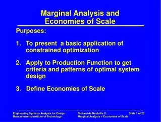
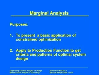
Marginal Analysis. Purposes: 1. To present a basic application of constrained optimization 2. Apply to Production Function to get criteria and patterns of optimal system design. Marginal Analysis: Outline. 1. Definition and Assumptions 2. Optimality criteria Analysis Interpretation

Marginal Analysis
E N D
Presentation Transcript
Marginal Analysis Purposes: 1. To present a basic application of constrained optimization 2. Apply to Production Function to get criteria and patterns of optimal system design
Marginal Analysis: Outline 1. Definition and Assumptions 2. Optimality criteria • Analysis • Interpretation • Application 3. Key concepts • Expansion path • Cost function • Economies of scale 4. Summary
Marginal Analysis: Concept • Basic form of optimization of design • Combines: Production function - Technical efficiency Input cost function, c(X) Economic efficiency
Marginal Analysis: Assumptions • Feasible region is convex (over relevant portion) This is key. Why? • To guarantee no other optimum missed • No constraints on resources • To define a general solution • Models are “analytic” (continuously differentiable) • Finds optimum by looking at margins -- derivatives
Fixed level of output vector of resources Optimality Conditionsfor Design, by Marginal Analysis The Problem: Min C(Y’) = c(X) cost of inputs for any level of output, Y’ s.t. g(X) = Y’ production function The Lagrangean: L = c(X) - [g(X) - Y’]
balanced design Optimality Conditions for Design: Results • Key Result: c(X) / Xi = g(X) / Xi • Optimality Conditions: MPi / MCi = MPj / MCj = 1 / MCj / MPj = MCi / MPi = = Shadow Price on Product • A Each Xi contributes “same bang for buck” marginal cost marginal product
X2 X1 Optimality Conditions: Graphical Interpretation of Costs (A) Input Cost Function Linear Case: B = Budget c(X) = piXi B B/P2 P2 General case: Budget is non-linear (as in curved line) P1 B/P1
Optimality Conditions: Graphical Interpretation of Results (B) Conditions Slope = MRSij = - MP1 / MP2 = - MC1 / MC2 X2 Isoquant $ X1
Note: Linearity of Input Cost Function - typically assumed by economists - in general, not valid prices rise with demand wholesale, volume discounts Application of Optimality Conditions -- Conventional Case Problem: Y = a0X1a1 X2a2 c(X) = piXi Solution: [a1 / X1*] Y / p1 = [a2 / X2*] Y / p2 ==> [a1 / X1*] p1 = [a2 / X2*] / p2 ( * denotes an optimum value)
Assume Y = 2X10.48 X20.72 (increasing RTS) c(X) = 5X1 + 3X2 Apply Conditions: = MPi / MCi [a1 / X1*] / p1 = [a2 / X2*] / p2 [0.48 /5] / X1* = [ 0.72/ 3] / X2* 9.6 / X1* = 24 / X2* This can be solved for a general relationship between resources => Expansion Path Optimality Conditions: Example
Expansion Path • Locus of all optimal designs X* • Not a property of technical system alone • Depends on local prices • Optimal designs do not, in general, maintain constant ratios between optimal Xi* Compare: crew of 20,000 ton ship crew of 200,000 ton ship larger ship does not need 10 times as many sailors as smaller ship
X2 Y Expansion Path X1 Expansion Path: Non-Linear Prices • Assume: Y = 2X10.48 X20.72 (increasing RTS) c(X) = X1 + X21.5 (increasing costs) • Optimality Conditions: (0.48 / X1) Y / 1 = (0.72 / X2) Y / (1.5X20.5) => X1* = (X2*)1.5 • Graphically:
Cost Functions: Concept • Not same as input cost function It represents the optimal cost of Y Not the cost of any set of X • C(Y) = C(X*) = f (Y) • It is obtained by inserting optimal values of resources (defined by expansion path) into input cost and production functions to give “best cost for any output”
Engineer’s view Cost-Effectiveness Economist’s view Cost Functions: Graphical View • Graphically: • Great practical use: How much Y for budget? Y for B? Cost effectiveness, B / Y C(Y) Y Feasible Feasible Y C(Y)
Cost Function Calculation: Linear Costs • Cobb-Douglas Prod. Fcn: Y = a0Xiai • Linear input cost function: c(X) = piXi • Result • C(Y) = A(piai/r)Y1/r where r = ai • Easy to estimate statistically => Solution for ‘ai’ => Estimate of prod. fcn. Y = a0Xiai
Cost Function Calculation: Example • Assume Again: Y = 2X10.48 X20.72 c(X) = X1 + X21.5 • Expansion Path: X1* = (X2*)1.5 • Thus: Y = 2(X2*)1.44 c(X*) = 2(X2*)1.5 => X2* = (Y/2)0.7 c(Y) = c(X*) = (2-0.05)Y1.05
Real Example: Communications Satellites • System Design for Satellites at various altitudes and configurations • Source: O. de Weck and MIT co-workers • Data generated by a technical model that costs out wide variety of possible designs • Establishes a Cost Function • Note that we cannot in general expand along cost frontier. Technology limits what we can do: Only certain pathways are available
Key Parameters • Each star in the Trade Space corresponds to a vector: • r: altitude of the satellites - e: minimum acceptable elevation angle • C: constellation type • Pt: maximal transmitter power • DA: Antenna diameter - Dfc: bandwidth • ISL: intersatellite links • Tsat: Satellites lifetime • Some are fixed: • C: polar - Dfc: 40 kHz
Path example • r= 400 km • = 35 deg Nsats=1215 Lifecycle cost [B$] Constants: Pt=200 W DA=1.5 m ISL= Yes Tsat= 5 • r= 400 km • = 20 deg Nsats=416 • r= 2000 km • = 5 deg Nsats=24 • r= 800 km • = 5 deg Nsats=24 • r= 400 km • = 5 deg Nsats=112 System Lifetime capacity [min]
Tree example • r= 400 km • = 35 deg N= 1215 Lifecycle cost [B$] Constants: Pt=200 W DA=1.5 m ISL= Yes Tsat= 5 e = 35 deg e = 20 deg • r= 2000 km • = 5 deg N=24 System Lifetime capacity [min]
Economies of Scale: Concept • A possible characteristic of cost function • Concept similar to returns to scale, except • ratio of ‘Xi’ not constant • refers to costs (economies) not “returns” • Not universal (as RTS) but depends on local costs • Economies of scale exist if costs increase slower than product Total cost = C(Y) = Y < 1.0
Economies of Scale: Specific Cases • If Cobb-Douglas, linear input costs, Increasing RTS (r = ai > 1.0 => Economies of scale Optimality Conditions: [a1/X1*] / p1 = [a2/X2*] / p2 Thus: Inputs Cost is a function of X1* Also: Output is a function of [X1* ] r So: X1* is a function of Y1/r Finally: C(Y) = function of [ Y1/r ]
Economies of Scale: General Case Not necessarily true in general that Returns to scale => Economies of Scale Increasing costs may counteract advantages of returns to scale See example!! c(Y) = c(X*) = (2-0.05)Y1.05 Contrarily, if unit prices decrease with volume (quite common) we can have Economies of Scale, without Returns to Scale
Marginal Analysis: Summary • Assumptions -- -- convex feasible region -- Unconstrained • Optimality Criteria • MC/MP same for all inputs • Expansion path -- Locus of Optimal Design • Cost function -- cost along Expansion Path • Economies of scale (vs Returns to Scale) -- Exist if Cost/Unit decreases with volume