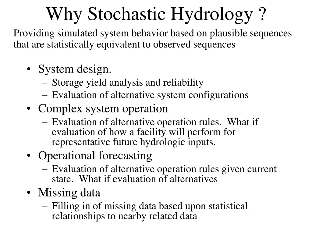
Why Stochastic Hydrology ?

1. Why Stochastic Hydrology ? Providing simulated system behavior based on plausible sequences that are statistically equivalent to observed sequences • System design. • Storage yield analysis and reliability • Evaluation of alternative system configurations • Complex system operation • Evaluation of alternative operation rules. What if evaluation of how a facility will perform for representative future hydrologic inputs. • Operational forecasting • Evaluation of alternative operation rules given current state. What if evaluation of alternatives • Missing data • Filling in of missing data based upon statistical relationships to nearby related data

2. The Monte Carlo Simulation Approach • Streamflow and other hydrologic time series inputs are random (resulting from lack of knowledge and unknowability of boundary conditions and inputs) • System behavior is complex • Can be represented by a simulation model • Analytic derivation of probability distribution of system output is intractable • Inputs generated from a Monte Carlo simulation model designed to capture the essential statistical structure of the input time series • Monte Carlo simulations solve the derived distribution problem to allow numerical determination of probability distributions of output variables

3. From Bras, R. L. and I. Rodriguez-Iturbe, (1985), Random Functions and Hydrology, Addison-Wesley, Reading, MA, 559 p.

4. Streamflow Modeling • A stochastic streamflow model should reproduce what are judged to be the fundamental characteristics of the joint distribution of the flows. • What characteristics are important to reproduce?

5. Marginal Distributions • Mean • Std Deviation • Skewness • Extremes • Full distribution • Normalizing transformations • Box-cox • Parametric PDF • Nonparametric PDF • Measures of fit • Kolmogorov smirnoff • Probability plot correlation (Filliben) • Shapiro-Wilks • Likelihood

6. Parametric vs Nonparametric • Parametric • Assume data from a known distribution (e.g. Gamma, Normal) and estimate parameters • Nonparametric • Assume that the data has a probability density function but not of a specific known form • Let data speak for themselves • Exploratory data analysis

7. Kernel Density Estimate (KDE) • Place “kernels” at each data point • Sum up the kernels • Width of kernel determines level of smoothing • Determining how to choose the width of the kernel is an important topic! Narrow kernel Medium kernel Wide kernel

8. KDE window width sensitivity

9. Normalizing transformation for arbitrary distribution Normal distribution Fn(y) Arbitrary distribution F(x) y x Normalizing transformation Back transformation

10. Relationships between variables • Correlation • Autocorrelation • Partial autocorrelation • State dependent correlation • Cross correlation • Spectral density

11. Storage related Threshold related • Storage-yield • Reliability • Range and Hurst coefficient • Duration above/below • Accumulation above/below

12. Lake Powell Capacity 27 MAF

13. General form of a stochastic hydrology model Qt=F(Qt-1, Qt-2, …, random inputs) Example Regression of later values against earlier values

14. General function fitting

15. Time series function fitting x1 x2 . . xt . .

16. Time series autoregressive function fitting – Method of delays Embedding dimension x1 x2 x3 x4 x2 x3 x4 x5 x3 x4 x5 x6 ……… xt-3 xt-2 xt-1 xt ……… Samples data vectors constructed using lagged copies of the single time series ExampleAR1 model xt =  xt-1 +  Trajectory matrix

17. Multiple Random Variables and Joint Distributions • The conditional dependence between random variables serves as a foundation for time series analysis. • When multiple random variables are related they are described by their joint distribution and density functions

19. Conditional and joint density functions Conditional density function Marginal density function If X and Y are independent

20. Marginal Distribution

21. Conditional Distribution

22. The theoretical basis for time series models • A random process is a sequence of random variables indexed in time • A random process is fully described by defining the (infinite) joint probability distribution of the random process at all times

23. xt+1 = g(xt, xt-1, …,) + random innovation (errors or unknown random inputs) Random Processes • A sequence of random variables indexed in time • Infinite joint probability distribution

24. From Sharma et al., 1997

25. Disaggregation From Loucks et al., 1981

26. Nonparametric disaggregation From Tarboton et al., 1998

27. Spectral representation of a stationary random process Autocorrelation Autocorrelation function Time Series Fourier Transform Fourier Transform Spectral density function Fourier coefficients Smoothing

28. Spectral analysis gives us • Decomposition of process into dominant frequencies • Diagnosis and detection of periodicities and repeatable patterns • Capability to, through sampling from the spectrum, simulate a process with any S(w) and hence any Cov() • By comparison of input and output spectra infer aspects of the process based on which frequencies are attenuated and which propagate through

29. Limitations of Stochastic Hydrology • Stochastic Hydrology can not create more information than already exists in the available data. What it does do is provide a methodology to help decision makers find the answers to "what if" questions by providing simulated system behavior based on plausible sequences that mimic the records that are already available (Pegram, 1989)

30. Why Stochastic Hydrology • Because although future rainfalls and streamflows will most likely resemble the past in a broad sense (such as mean values, variability and intercorrelation) all future sequences are almost surely going to be different in detail from what has been observed in the past (Pegram, 1989)