Feedforward and Ratio Control
450 likes | 859 Vues
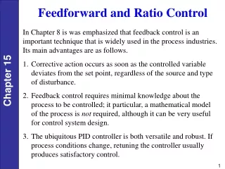
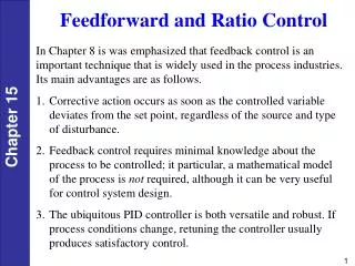
In Chapter 8 is was emphasized that feedback control is an important technique that is widely used in the process industries. Its main advantages are as follows. Feedforward and Ratio Control.

Feedforward and Ratio Control
E N D
Presentation Transcript
In Chapter 8 is was emphasized that feedback control is an important technique that is widely used in the process industries. Its main advantages are as follows. • Feedforward and Ratio Control • Corrective action occurs as soon as the controlled variable deviates from the set point, regardless of the source and type of disturbance. • Feedback control requires minimal knowledge about the process to be controlled; it particular, a mathematical model of the process is not required, although it can be very useful for control system design. • The ubiquitous PID controller is both versatile and robust. If process conditions change, retuning the controller usually produces satisfactory control.
However, feedback control also has certain inherent disadvantages: • No corrective action is taken until after a deviation in the controlled variable occurs. Thus, perfect control, where the controlled variable does not deviate from the set point during disturbance or set-point changes, is theoretically impossible. • Feedback control does not provide predictive control action to compensate for the effects of known or measurable disturbances. • It may not be satisfactory for processes with large time constants and/or long time delays. If large and frequent disturbances occur, the process may operate continuously in a transient state and never attain the desired steady state. • In some situations, the controlled variable cannot be measured on-line, and, consequently, feedback control is not feasible.
Introduction to Feedforward Control The basic concept of feedforward control is to measure important disturbance variables and take corrective action before they upset the process. Feedforward control has several disadvantages: • The disturbance variables must be measured on-line. In many applications, this is not feasible. • To make effective use of feedforward control, at least a crude process model should be available. In particular, we need to know how the controlled variable responds to changes in both the disturbance and manipulated variables. The quality of feedforward control depends on the accuracy of the process model. • Ideal feedforward controllers that are theoretically capable of achieving perfect control may not be physically realizable. Fortunately, practical approximations of these ideal controllers often provide very effective control.
Figure 15.2 The feedback control of the liquid level in a boiler drum.
A boiler drum with a conventional feedback control system is shown in Fig. 15.2. The level of the boiling liquid is measured and used to adjust the feedwater flow rate. • This control system tends to be quite sensitive to rapid changes in the disturbance variable, steam flow rate, as a result of the small liquid capacity of the boiler drum. • Rapid disturbance changes can occur as a result of steam demands made by downstream processing units. The feedforward control scheme in Fig. 15.3 can provide better control of the liquid level. Here the steam flow rate is measured, and the feedforward controller adjusts the feedwater flow rate.
Figure 15.3 The feedforward control of the liquid level in a boiler drum.
Figure 15.4 The feedfoward-feedback control of the boiler drum level.
In practical applications, feedforward control is normally used in combination with feedback control. • Feedforward control is used to reduce the effects of measurable disturbances, while feedback trim compensates for inaccuracies in the process model, measurement error, and unmeasured disturbances. Ratio Control Ratio control is a special type of feedforward control that has had widespread application in the process industries. The objective is to maintain the ratio of two process variables as a specified value. The two variables are usually flow rates, a manipulated variable u, and a disturbance variable d. Thus, the ratio is controlled rather than the individual variables. In Eq. 15-1, u and d are physical variables, not deviation variables.
Typical applications of ratio control include: • Setting the relative amounts of components in blending operations • Maintaining a stoichiometric ratio of reactants to a reactor • Keeping a specified reflux ratio for a distillation column • Holding the fuel-air ratio to a furnace at the optimum value.
The main advantage of Method I is that the actual ratio R is calculated. • A key disadvantage is that a divider element must be included in the loop, and this element makes the process gain vary in a nonlinear fashion. From Eq. 15-1, the process gain is inversely related to the disturbance flow rate . Because of this significant disadvantage, the preferred scheme for implementing ratio control is Method II, which is shown in Fig. 15.6.
Regardless of how ratio control is implemented, the process variables must be scaled appropriately. • For example, in Method II the gain setting for the ratio station Kd must take into account the spans of the two flow transmitters. • Thus, the correct gain for the ratio station is where Rd is the desired ratio, Su and Sd are the spans of the flow transmitters for the manipulated and disturbance streams, respectively.
Example 15.1 A ratio control scheme is to be used to maintain a stoichoimetric ratio of H2 and N2 as the feed to an ammonia synthesis reactor. Individual flow controllers will be used for both the H2 and N2 streams. Using the information given below, do the following: • Draw a schematic diagram for the ratio control scheme. • Specify the appropriate gain for the ratio station, KR.
Available Information • The electronic flow transmitters have built-in square root extractors. The spans of the flow transmitters are 30 L/min for H2 and 15 L/min for N2. • The control valves have pneumatic actuators. • Each required current-to-pressure (I/P) transducer has a gain of 0.75 psi/mA. • The ratio station is an electronic instrument with 4-20 mA input and output signals. Solution The stoichiometric equation for the ammonia synthesis reaction is
In order to introduce the feed mixture in stoichiometric proportions, the ratio of the molar flow rates (H2/N2) should be 3:1. For the sake of simplicity, we assume that the ratio of the molar flow rates is equal to the ratio of the volumetric flow rates. But in general, the volumetric flow rates also depend on the temperature and pressure of each stream (cf., the ideal gas law). • The schematic diagram for the ammonia synthesis reaction is shown in Fig. 15.7. The H2 flow rate is considered to be the disturbance variable, although this choice is arbitary because both the H2 and N2 flow rates are controlled. Note that the ratio station is merely a device with an adjustable gain. The input signal to the ratio station is dm, the measured H2 flow rate. Its output signal usp serves as the set point for the N2 flow control loop. It is calculated as usp = KRdm.
Figure 15.7 Ratio control scheme for an ammonia synthesis reactor of Example 15.1
From the stoichiometric equation, it follows that the desired ratio is Rd = u/d = 1/3. Substitution into Equation 15-3 gives: Feedforward Controller Design Based on Steady-State Models • A useful interpretation of feedforward control is that it continually attempts to balance the material or energy that must be delivered to the process against the demands of the load. • For example, the level control system in Fig. 15.3 adjusts the feedwater flow so that it balances the steam demand. • Thus, it is natural to base the feedforward control calculations on material and energy balances.
Figure 15.8 A simple schematic diagram of a distillation column.
To illustrate the design procedure, consider the distillation column shown in Fig. 15.8 which is used to separate a binary mixture. • In Fig. 15.8, the symbols B, D, and F denote molar flow rates, whereas x, y, and z are the mole fractions of the more volatile component. • The objective is to control the distillation composition, y, despite measurable disturbances in feed flow rate F and feed composition z, by adjusting distillate flow rate, D. • It is assumed that measurements of x and y are not available. The steady-state mass balances for the distillation column can be written as
Solving (15-4) for D and substituting into (15-5) gives Because x and y are not measured, we replace these variables by their set points to yield the feedforward control law:
Blending System • Consider the blending system and feedforward controller shown in Fig. 15.9. • We wish to design a feedforward control scheme to maintain exit composition x at a constant set point xsp, despite disturbances in inlet composition, x1. • Suppose that inlet flow rate w1and the composition of the other inlet stream, x2, are constant. • It is assumed that x1ismeasured but x is not.
Figure 15.9 Feedforward control of exit composition in the blending system.
The starting point for the feedforward controller design is the steady-state mass and component balances, where the bar over the variable denotes a steady-state value. Substituting Eq. 15-8 into 15-9 and solving for gives: In order to derive a feedforward control law, we replace by xsp, and and , by w2(t) and x1(t), respectively: Note that this feedforward control law is based on the physical variables rather than on the deviation variables.
The feedforward control law in Eq. 15-11 is not in the final form required for actual implementation because it ignores two important instrumentation considerations: • First, the actual value of x1is not available but its measured value, x1m, is. • Second, the controller output signal is p rather than inlet flow rate, w2. • Thus, the feedforward control law should be expressed in terms of x1mand p,rather than x1 and w2. • Consequently, a more realistic feedforward control law should incorporate the appropriate steady-state instrument relations for the w2 flow transmitter and the control valve. (See text.)
Feedforward Controller Design Based on Dynamic Models In this section, we consider the design of feedforward control systems based on dynamic, rather than steady-state, process models. • As a starting point for our discussion, consider the block diagram shown in Fig. 15.11. • This diagram is similar to Fig. 11.8 for feedback control but an additional signal path through Gtand Gf has been added.
Figure 15.11 A block diagram of a feedforward-feedback control system.
The closed-loop transfer function for disturbance changes is: Ideally, we would like the control system to produce perfect control where the controlled variable remains exactly at the set point despite arbitrary changes in the disturbance variable, D. Thus, if the set point is constant (Ysp(s) = 0), we want Y(s) = 0, even though D(s) • Figure 15.11 and Eq. 15-21 provide a useful interpretation of the ideal feedforward controller. Figure 15.11 indicates that a disturbance has two effects. • It upsets the process via the disturbance transfer function, Gd; however, a corrective action is generated via the path through GtGfGvGp.
Ideally, the corrective action compensates exactly for the upset so that signals Yd and Yu cancel each other and Y(s) = 0. Example 15.2 Suppose that Then from (15-22), the ideal feedforward controller is This controller is a lead-lag unit with a gain given by Kf = -Kd/KtKvKp. The dynamic response characteristics of lead-lag units were considered in Example 6.1 of Chapter 6.
Example 15.3 Now consider From (15-21), Because the term is a negative time delay, implying a predictive element, the ideal feedforward controller in (15-25) is physically unrealizable. However, we can approximate it by omitting the term and increasing the value of the lead time constant from to .
Example 15.4 Finally, if then the ideal feedforward controller, is physically unrealizable because the numerator is a higher order polynomial in s than the denominator. Again, we could approximate this controller by a physically realizable one such as a lead-lag unit, where the lead time constant is the sum of the two time constants,
Stability Considerations • To analyze the stability of the closed-loop system in Fig. 15.11, we consider the closed-loop transfer function in Eq. 15-20. • Setting the denominator equal to zero gives the characteristic equation, • In Chapter 11 it was shown that the roots of the characteristic equation completely determine the stability of the closed-loop system. • Because Gf does not appear in the characteristic equation, the feedforward controller has no effect on the stability of the feedback control system. • This is a desirable situation that allows the feedback and feedforward controllers to be tuned individually.
Lead-Lag Units • The three examples in the previous section have demonstrated that lead-lag units can provide reasonable approximations to ideal feedforward controllers. • Thus, if the feedforward controller consists of a lead-lag unit with gain Kf, we can write Example 15.5 Consider the blending system of Section 15.3 and Fig. 15.9. A feedforward-feedback control system is to be designed to reduce the effect of disturbances in feed composition, x1, on the controlled variable, produce composition, x. Inlet flow rate, w2, can be manipulated. (See text.)
Configurations for Feedforward-Feedback Control In a typical control configuration, the outputs of the feedforward and feedback controllers are added together, and the sum is sent as the signal to the final control element. Another useful configuration for feedforward-feedback control is to have the feedback controller output serve as the set point for the feedforward controller.
Figure 15.14 Feedforward-feedback control of exit composition in the blending system.
Figure 15.15 The open-loop responses to step changes in u and d.
Tuning Feedforward Controllers Feedforward controllers, like feedback controllers, usually require tuning after installation in a plant. Step 1. Adjust Kf. • The effort required to tune a controller is greatly reduced if good initial estimates of the controller parameters are available. • An initial estimate of Kf can be obtained from a steady-state model of the process or steady-state data. • For example, suppose that the open-loop responses to step changes in d and u are available, as shown in Fig. 15.15. • After Kp and Kd have been determined, the feedforward controller gain can be calculated from the steady-state version of Eq. 15-22:
To tune the controller gain, Kfis set equal to an initial value, and a small step change (3 to 5%) in the disturbance variable d is introduced, if this is feasible. • If an offset results, then Kf is adjusted until the offset is eliminated. • While Kf is being tuned, and should be set equal to their minimum values, ideally zero. Step 2. Determine initial values for and . • Theoretical values for and can be calculated if a dynamic model of the process is available, as shown in Example 15.2. • Alternatively, initial estimates can be determined from open-loop response data. • For example, if the step responses have the shapes shown in Figure 15.16, a reasonable process model is
where and can be calculated as shown in Fig. 15.16. • A comparison of Eqs. 15-24 and 5-30 leads to the following expression for and : • These values can then be used as initial estimates for the fine tuning of and in Step 3. • If neither a process model nor experimental data are available, the relations or may be used, depending on whether the controlled variable responds faster to the load variable or to the manipulated variable.
In view of Eq. 15-58, should be set equal to the estimated dominant process time constant. Step 3. Fine tune and . • The final step is to use a trial-and-error procedure to fine tune and by making small step changes in d. • The desired step response consists of small deviations in the controlled variable with equal areas above and below the set point [1], as shown in Fig. 15.17. • For simple process models, it can be proved theoretically that equal areas above and below the set point imply that the difference, , is correct (Exercise 15.8). • In subsequent tuning to reduce the size of the areas, and should be adjusted so that remains constant.
Figure 15.16 The desired response for a well-tuned feedforward controller. (Note approximately equal areas above and below the set point.)
As a hypothetical illustration of this trial-and-error tuning procedure, consider the set of responses shown in Fig. 15.17 for positive step changes in disturbance variable d. It is assumed that Kp > 0, Kd < 0, and controller gain Kf has already been adjusted so that offset is eliminated.