An Earth System Model based on the ECMWF Integrated Forecasting System

1. An Earth System Model based on the ECMWF Integrated Forecasting System IFS-model What is the IFS? Governing equations Dynamics and physics Numerical implementation Overview of the code

2. What is the IFS? • Total software package at ECMWF: • Data-assimilation to get initial condition • Make weather forecasts • Make ensemble forecasts • Monthly forecasts • Seasonal forecasts • Atmosphere, ocean, land, wave models • Has a long history that is present in the code ….

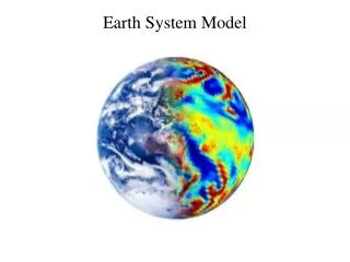
3. Numerical Weather Prediction • The behaviour of the atmosphere is governed by a set of physical laws • Equations cannot be solved analytically, numerical methods are needed • Additionally, knowledge of initial conditions of system necessary • Incomplete picture from observations can be completed by data assimilation • Interactions between atmosphere and land/ocean important

4. ECMWF’s operational analysis and forecasting system The comprehensive earth-system model developed at ECMWF forms the basis for all the data assimilation and forecasting activities. All the main applications required are available through one integrated computer software system (a set of computer programs written in Fortran) called the Integrated Forecast System or IFS • Numerical scheme:  TL799L91 (799 waves around a great circle on the globe, 91 levels 0-80 km) semi-Lagrangian formulation 1,630,000,000,000,000 computations required for each 10-day forecast • Time step:  12 minutes • Prognostic variables:  wind, temperature, humidity, cloud fraction and water/ice content, pressure at surface grid-points, ozone • Grid:  Gaussian grid for physical processes, ~25 km, 76,757,590 grid points

5. A history Resolution increases of the deterministic 10-day medium-range Integrated Forecast System (IFS) over ~25 years at ECMWF: 1987: T 106 (~125km) 1991: T 213 (~63km) 1998: TL319 (~63km) 2000: TL511 (~39km) 2006: TL799 (~25km) 2010: TL1279 (~16km) 2015?: TL2047 (~10km) 2020-???: (~1-10km) Non-hydrostatic, cloud-permitting, substan-tially different cloud-microphysics and turbulence parametrization, substantially different dynamics-physics interaction ?

6. Ultra-high resolution global IFS simulations TL0799 (~ 25km) >> 843,490 points per field/level TL1279 (~ 16km) >> 2,140,702 points per field/level TL2047 (~ 10km) >> 5,447,118 points per field/level TL3999 (~ 5km) >> 20,696,844 points per field/level (world record for spectral model ?!)

7. Orography – T1279 Max global altitude = 6503m Alps

8. Orography - T3999 Max global altitude = 7185m Alps

9. Deterministic model grid (T799)

10. EPS model grid (T399)

11. The wave model • Coupled ocean wave model (WAM cycle4)  2 versions: global and regional (European Shelf & Mediterranean)  numerical scheme: irregular lat/lon grid, 40 km spacing; spectrum with 30 frequencies and 24 directions  coupling: wind forcing of waves every 15 minutes, two way interaction of winds and waves, sea state dep. drag coefficient  extreme sea state forecasts: freak waves  wave model forecast results can be used as a tool to diagnose problems in the atmospheric model Numerical Methods and Adiabatic Formulation of Models 30 March - 3 April 2009

12. Physical aspects, included in IFS • Orography (terrain height and sub-grid-scale characteristics) • Four surface and sub-surface levels (allowing for vegetation cover, gravitational drainage, capillarity exchange, surface / sub-surface runoff) • Stratiform and convective precipitation • Carbon dioxide (345 ppmv fixed), aerosol, ozone • Solar angle • Diffusion • Ground & sea roughness • Ground and sea-surface temperature • Ground humidity • Snow-fall, snow-cover and snow melt • Radiation (incoming short-wave and out-going long-wave) • Friction (at surface and in free atmosphere) • Sub-grid-scale orographic drag • Gravity waves and blocking effects • Evaporation, sensible and latent heat flux Parameterization of Diabatic Processes 11 – 21 May 2009

13. Starting a forecast: The initial conditions

14. Data Assimilation • Observations measure the current state, but provide an incomplete picture  Observations made at irregularly spaced points, often with large gaps  Observations made at various times, not all at ‘analysis time’  Observations have errors  Many observations not directly of model variables • The forecast model can be used to process the observations and produce a more complete picture (data assimilation)  start with previous analysis  use model to make short-range forecast for current analysis time  correct this ‘background’ state using the new observations

15. Analysis 12-hour forecast Data Assimilation Background Analysis Observations Every 12 hours ~ 60 million observations are processed to correct the 8 million numbers that define the model’s virtual atmosphere Model variables, e.g. temperature “True” state of the atmosphere 12 UTC 5 May 00 UTC 6 May 12 UTC 6 May 00 UTC 5 May

16. Data Assimilation • Observations measure the current state, but provide an incomplete picture  Observations made at irregularly spaced points, often with large gaps  Observations made at various times, not all at ‘analysis time’  Observations have errors  Many observations not directly of model variables • The forecast model can be used to process the observations and produce a more complete picture (data assimilation)  start with previous analysis  use model to make short-range forecast for current analysis time  correct this ‘background’ state using the new observations • The forecast model is very sensitive to small differences in initial conditions  accurate analysis crucial for accurate forecast  EPS used to represent the remaining analysis uncertainty

17. What is an ensemble forecast? Temperature Forecast time Initial condition Forecast Complete description of weather prediction in terms of a Probability Density Function (PDF)

18. Flow dependence of forecast errors 26th June 1995 26th June 1994 If the forecasts are coherent (small spread) the atmosphere is in a more predictable state than if the forecasts diverge (large spread)

19. ECMWF’s Ensemble Prediction Systems • Account for initial uncertainties by running ensemble of forecasts from slightly different initial conditions  singular vector approach to sample perturbations • Model uncertainties are represented by “stochastic physics” • Medium-range VarEPS (15-day lead) runs twice daily (00 and 12 UTC)  day 0-10: TL399L62 (0.45°, ~50km), 50+1 members  day 9-15: TL255L62 (0.7°, ~80km), 50+1 members • Extended time-range EPS systems: monthly and seasonal forecasts  coupled atmosphere-ocean model (IFS & HOPE)  monthly forecast (4 weeks lead) runs once a week  seasonal forecast (6 months lead) runs once a month

20. Principal Goal

21. Forecast errors Two kinds of forecast error • Random error (model+initial error) • Systematic error (model error*) Two principal sources of forecast error: • Uncertainties in the initial conditions (“observational error”) • Model error

22. Systematic Error Growth How do systematic errors grow throughout the forecast?

23. Systematic Z500 Error Growth from D+1 to D+10

24. Systematic Z500 Errors: Medium-Range and Beyond Asymptotic: 31R2 D+10 ERA-Interim

25. Evolution of Systematic Error How did systematic errors evolve throughout the years?

26. Evolution of D+3 Systematic Z500 Errors 1983-1987 1993-1997 2003-2007

27. Evolution of Systematic Z500 Errors: Model Climate 35R1 33R1 32R3 32R2 32R1 31R1 30R1 29R2

28. Systematic Z500 Errors: Impact of Recent Changes Control Old Convection Old TOFD Old Vertical Diff Old Radiation Old Soil Hydrology

29. Recent Model Changes

30. An Earth System Model based on the ECMWF Integrated Forecasting System IFS-model What is the IFS? Governing equations Dynamics and physics Numerical implementation Overview of the code

31. Primitive (hydrostatic) equations in IFS Momentum equations for Sub-grid model : “physics” Numerical diffusion

32. IFS hydrostatic equations Thermodynamic equation Moisture equation Note: virtual temperature Tv instead of T from the equation of state.

33. IFS hydrostatic equations Continuity equation Vertical integration of the continuity equation in hybrid coordinates

34. One word about water species…. Phase changes are treated inside the “physics” (P terms) But the prognostic water species have a weight. They are included in the full density of the moist air and in the definition of the “specific” variables. It does some “tricky” changes in the equations. For ex. : Prognostic water species should be advected. They are then also treated by the dynamics. Perfect gas equation

35. An Earth System Model based on the ECMWF Integrated Forecasting System IFS-model What is the IFS? Governing equations Dynamics and physics Numerical implementation Overview of the code

36. Resolution problem So far : We derived a set of evolution equations based on 3 basic conservation principles valid at the scale of the continuum : continuity equation, momentum equation and thermodynamic equation. What do we want to (re-)solve in models based on these equations? The scale of the grid is much bigger than the scale of the continuum resolved scale (?) grid scale

37. “Averaged” equations : from the scale of the continuum to the mean grid size scale The equations as used in an operational NWP model represent the evolution of a space-time average of the true solution. The equations become empirical once averaged, we cannot claim we are solving the fundamental equations. Possibly we do not have to use the full form of the exact equations to represent an averaged flow, e.g. hydrostatic approximation OK for large enough averaging scales in the horizontal.

38. Different scales involved NH-effects visible

39. “Averaged” equations The sub-grid model represents the effect of the unresolved scales on the averaged flow expressed in terms of the input data which represents an averaged state. The mean effects of the subgrid scales has to be parametrised. The average of the exact solution may *not* look like what we expect, e.g. since vertical motions over land may contain averages of very large local values. The averaging scale does not correspond to a subset of observed phenomena, e.g. gravity waves are partly included at TL799, but will not be properly represented.

40. Physics – Dynamics coupling ‘Physics’, parametrization: “the mathematical procedure describing the statistical effect of subgrid-scale processes on the mean flow expressed in terms of large scale parameters”, processes are typically:vertical diffusion, orography, cloud processes, convection, radiation ‘Dynamics’: “computation of all the other terms of the Navier-Stokes equations (eg. in IFS: semi-Lagrangian advection)” The ‘Physics’ in IFS is currently formulated inherently hydrostatic, because the parametrizations are formulated as independent vertical columns on given pressure levels and pressure is NOT changed directly as a result of sub-gridscale interactions ! The boundaries between ‘Physics’ and ‘Dynamics’ are “a moving target” …

41. An Earth System Model based on the ECMWF Integrated Forecasting System IFS-model What is the IFS? Governing equations Dynamics and physics Numerical implementation Overview of the code

42. Fundamentals of series-expansion methods We demonstrate the fundamentals of series-expansion methods on the following problem for which we seek solutions: Partial differential equation: (with an operator H involving only derivatives in space.) (1) To be solved on the spatial domain S subject to specified initial and boundary conditions. Initial condition: (1a) Boundary conditions: Solution f has to fulfil some specified conditions on the boundary of the domain S.

43. The set of expansion function should span the L2 space, i.e. a Hilbert space with the inner (or scalar) product of two functions defined as Fundamentals of series-expansion methods (cont) The basic idea of all series-expansion methods is to write the spatial dependence of f as a linear combination of known expansion functions (3) (4) The expansion functions should all satisfy the required boundary conditions.

44. is only an approximation to the true solution f of the equation (1). The task of solving (1) has been transformed into the problem of finding the unknown coefficients in a way that minimises the error in the approximate solution. Fundamentals of series-expansion methods (cont) Numerically we can’t handle infinite sums. Limit the sum to a finite number of expansion terms N (3a) =>

45. =0 (Galerkin approximation) (9) Fundamentals of series-expansion methods (cont) Transform equation (1) into series-expansion form: Start from equation (5) (equivalent to (1)) (5) Take the scalar product of this equation with all the expansion functions and apply the Galerkin approximation: =>

46. The Spectral Method on the Sphere Spherical Harmonics Expansion Spherical geometry: Use spherical coordinates: longitude latitude Any horizontally varying 2d scalar field can be efficiently represented in spherical geometry by a series of spherical harmonic functions Ym,n: (40) (41) associated Legendre functions Fourier functions

47. This definition is only valid for ! The Spectral Method on the Sphere Definition of the Spherical Harmonics Spherical harmonics (41) The associated Legendre functionsPm,n are generated from the Legendre Polynomials via the expression (42) Where Pn is the “normal” Legendre polynomial of order n defined by (43)

48. The Spectral Method on the Sphere Some Spherical Harmonics for n=5

49. Schematic representation of the spectral transform method in the ECMWF model Grid-point space -semi-Lagrangian advection -physical parametrizations -products of terms FFT Inverse FFT Fourier space Fourier space Inverse LT LT Spectral space -horizontal gradients -semi-implicit calculations -horizontal diffusion FFT: Fast Fourier Transform, LT: Legendre Transform

50. Cubic B-splines as basis elements Basis elements for the representation of the integral F Basis elements for the represen- tation of the function to be integrated (integrand) f