Download
1 / 45
450 likes | 604 Vues
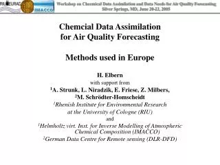
Chemcial Data Assimilation for Air Quality Forecasting Methods used in Europe. H. Elbern with support from 1 A. Strunk, L. Niradzik, E. Friese, Z. Milbers, 2 M. Schrödter-Homscheidt 1 Rhenish Institute for Environmental Research at the University of Cologne (RIU) and

E N D
Chemcial Data Assimilation for Air Quality ForecastingMethods used in Europe H. Elbern with support from 1A. Strunk, L. Niradzik, E. Friese, Z. Milbers, 2M. Schrödter-Homscheidt 1Rhenish Institute for Environmental Research at the University of Cologne (RIU) and 1Helmholtz virt. Inst. for Inverse Modelling of Atmospheric Chemical Composition (IMACCO) 2German Data Centre for Remote sensing (DLR-DFD)
Contents: • Survey and scope • Air Quality data assimilation in routine operations today • Advanced scientific applications • Kalman filter • 4dimensional variational data assimilation (4Dvar) • Example applications 4. Future research directions • Short term (1-3 years) • Long term (> 3 years)
Survey (1) Regional operational data assimilation • to comply with EU legislation • core assimilation data of in situ type from observation networks operated by national or regional/state authorities • Air Quality considered as a high resolution problem limited area and nested models • 2 major European efforts in Global Environmental Monitoring and Security (GEMS = European GEOSS) • ESA funded PROMOTE (www.gse-promote.org) • EU funded GEMS (new!) 1 Survey an Scope
European metropolitan chemograms ozone NO2 PM10 1 Survey an Scope SO2 CO benzene
Prevair system in PROMOTE analysis and observations 17.6.05 forecast and observations 2 Routine operations Method: Kriging Reference: Blond et Vautard, JGR, 2003, 2004
EURAD system in PROMOTE analysis and observations 28.5.05 forecast and observations 2 Routine operations Method: 2 and 3Dvar Reference: Reduced version of Elbern and Schmidt, JGR, 2001
Survey (2)Global tropospheric partly operational • MOCAGE (Meteo France) 3DFGAT, (= 3Dvar with “First Guess at Appropriate Time”) • TM3-5 (KNMI) “Kalman filter” with parameterize covariance update, • TM3-BETHY (MPI-BGC) soil column variational (1 spatial D + time D) 2 Routine operations
Special challenges of tropospheric chemistry data assimilation The following problems prevail: • strong influence of manifold processes including emissions and deposition • spatially highly variable “chemical regimes” • chemical state observability (= “analyseability”) hampered by manifold hydrocarbon species • consistency with heterogeneous data sources: satellite data and in situ observations 3. Advanced Mthods General remarks This invokes the application space-time data assimilation algorithms preserving the BLUE property (Best Linear Unbiased Estimator)
Advanced spatio-temporal data assimilation:4D dimensional variational and Kalman filtering • Model not to passively accept external 3D analyses (probably engendering spurious relaxations) • Rather contribute with its dynamics/ chemical kinetics as constraint to estimate the most probable state or parameter values 3. Advanced Mthods General remarks • Best Linear Unbiased Estimate (BLUE) while using data and models consistently allows for Hypothesis testing
Advanced spatio-temporal methods used in tropospheric chemistry data assimilation • 4-dim variational data assimilation (4D-VAR, and versions: 4D physical space statistical analysis system (Amodei, 1995; Courtier, 1997); 4D-var incremental (Courtier et al, 1994)) • reduced complexity versions of the Kalman Filter: Reduced Rank Square root KF (RRSQKF, Verlaan and Heemink, 1997) , ensemble KF (Evensen, 1994), SEEK, SEIK, (Verron et al., 1999) Spacio-temporal BLUEs applied in tropospheric chemistry data assimilation: • 4D var: • with EURAD (Elbern and Schmidt, 1999, 2001), • with POLAIR (Issartel and Baverel, 2003) • RRSQKF • with LOTOS model (van Loon et al, 2000), • with EUROS model (Hanea et al. 2004) Remark: 3D BLUE algorithm analyses like those from Optimal Interpolation, once ingested into a model, do not result in a 4D BLUE analysis For example 3D-FGAT is not! 3. Advanced Mthods General remarks
emission biased model state only initial value opt. concentration true state joint opt. observations only emission rate opt. time Hypothesis: initial state and emission rates are least known 3. Advanced Mthods General remarks
Kalman filter, basic equations 3. Advanced Mthods Lakman filter
Reduced rank Kalman filter (basic idea) Appoximate covariance matrices Pb,a (n x n) by a product of suitably low ranked matrix Sb,a (n x p), and p << n . Same procedure for the system noise matrix Q with T (n x r). The forecast step remains unchanged. The forecast error covariance matrix rests on 2 x p model integrations only! The enlargement of p by r enforces periodic reductions of columns (with lowest ranked eigenvalues) 3. Advanced Mthods Lakman filter
Reduced rank Kalman filter (calculus) In practice, all calculations can be performed without actually calculating matrices P! Positive semi-definitenes is maintained! 3. Advanced Mthods Lakman filter
Air quality Kalman filter implementationsand comlexity reduction strategy applied • LOTOS model (van Loon et al., 2000) • reduced rank square root • EUROS model (Hanea et al., 2004) • ensemble • reduce rank square root 3. Advanced Mthods Lakman filter Methods used with optimisation of various parameters including emissions
Transport-diffusion-reaction equation and its adjoint 3. Advanced Mthods 4D var
In the troposphere for emission rates the product (paucity of knowledge*importance)is high 3. Advanced Mthods Lakman filter 3. Advanced Mthods 4D var 3. Advanced Mthods Lakman filter
Adjoint integration “backward in time”(slide from lecture 1) How to make the parameters of resolvents i M(ti-1,ti) available in reverse order??
The 4D variational method:Key development: construction of the adjoint code forward model (forward differential equation) backward model (backward differential equation) 3. Advanced Mthods 4D var algorithm (solver) adjoint algorithm (adjoint solver) code adjoint code
Source identificationby 4DvarPOLAIR model Issartel and BaverelEcole National de Ponts et Chausees (ENPC) 3. Advanced Mthods 4D var application Calculations of optimal retroplumes (Issartel and Baverel, ACP, 2003)
4D-var configuration Mesoscale EURAD 4D-var data assimilation system meteorological driver MM5 emission rates direct CTM fore- cast Initial values minimisation adjoint CTM EURAD emission model EEM emission 1. guess 3. Advanced Mthods 4D var application gradient observations analysis
Computational complexity estimate of the variational algorithm Nx*Ny*Nz spatial dimensions O(104-105) Nc # constituents O(100) NT # time steps of assimilation window O(10-100) No # operators O(10) const intermediate results O(104) 3. Advanced Mthods 4D var application
1. step 2. step 3. step 4. step 5. step 6. step 7. step 8. step 9. step intermediate storage Level 1 backward integration 2 level forward and backward integration scheme time direction forward integration 3. Advanced Mthods 4D var application disk intermediate storage Level 1 backward integration
Chemie horiz. Advekt y horiz. Advekt y horiz. Advekt x vert.. Advekt vert.. Advekt horiz. Advekt x vert. Diffusion vert. Diffusion Adjungierte Chemie Adjungierte horiz. Advekt x Adjungierte horiz. Advekt y Adjungierte vert. Advekt Adjungierte vert.Diffusion horiz. Advekt y horiz. Advekt x vert.. Advekt vert. Diffusion Chemie Adjungierte vert.Diffusion Adjungierte vert. Advekt Adjungierte horiz. Advekt y Adjungierte horiz. Advekt x horiz. Advekt y vert.. Advekt horiz. Advekt x vert. Diffusion storage sequence: level 2, operator split(each time step) intermediate storage Level 1 Chemie horiz. Advekt y horiz. Advekt y horiz. Advekt x vert.. Advekt vert.. Advekt horiz. Advekt x vert. Diffusion vert. Diffusion 3. Advanced Mthods 4D var application intermediate storage Level 2 Adjungierte Chemie Adjungierte horiz. Advekt x Adjungierte horiz. Advekt y Adjungierte vert. Advekt Adjungierte vert.Diffusion Chemie Adjungierte vert.Diffusion Adjungierte vert. Advekt Adjungierte horiz. Advekt y Adjungierte horiz. Advekt x horiz. Advekt y horiz. Advekt y horiz. Advekt x vert.. Advekt vert.. Advekt horiz. Advekt x vert. Diffusion vert. Diffusion
Computational resources requested • with a 14 h assimilation interval about 18 iterations requested • results in 12 CPU-hours with 121 processors of a T3E 3. Advanced Mthods 4D var application
Normalised diurnal cycle of anthropogenic surface emissions f(t)emission(t)=f(t;location,species,day) * v(location,species)day in {working day, Saturday, Sunday} v optimization parameter 3. Advanced Mthods 4D var application
7. August 8. August 1997 Semi-rural measurement site Eggegebirge + observations no optimisation initial value opt. 3. Advanced Mthods 4D var application emis. rate opt. joint emis + ini val opt. assimilation interval forecast
assimilation window forecast assimilation window forecast error statisticsbias (top), root mean square (bottom) 3. Advanced Mthods 4D var application
Which is the requested resolution?BERLIOZ grid designs and observational sites (20.21. 07.1998) Control and diagnostics Dx=6 km Dx=18 km Dx=2 km Dx=54 km
Some BERLIOZ examples of NOx assimilation NO 3. Advanced Mthods 4D var application NO2 • Time series for selected NOx stations (upper panel NO, lower panel NO2) on nest 2. • + observations, • - - no assimilation,____ N1 assimilation (18 km), ____N2 assimilation.(6 km), • grey shading: assimilated observations, others forecasted.
NO2, (xylene (bottom), CO (top), and SO2 (from left to right). Emission source estimates by inverse modellingOptimised emission factors for Nest 3 height layer ~32-~70m 3. Advanced Mthods 4D var application surface
Status: EURAD assimilation system prepared for 4D-var assimilation production run 1.7.31.12.2003 • Gas phase satellite observations • KNMI - NO2 tropospheric columns, SCIAMACHY averaging kernel assimilation • NNORSY neural network based ozone tropospheric columns (revised version based on GOME) • IMK - MIPAS upper troposphere • Aerosol phase satellite observations • DFD - PM10 bulk retrievals SCAMACHY-AATSR 3. Advanced Mthods 4D var application
NO2 tropospheric column assimilation IFE:Example: BERLIOZ episode 20.7.1998 GOME retieval Courtesy: A. Richter, IFE Bremen no assimilation 3. Advanced Mthods 4D var application with assimilation NOAA 14 11:51 UTC
IUP Bremen GOMEGOME forecast validationmodel/retrieval ratio for BERLIOZ 20. (assimilated) + 21.(forecasted) 7.1998 no assimilation with assimilation 20.7.98 ideal 3. Advanced Mthods 4D var application forecast forecast verification forecast 21.7.98 (not assimilated)
KNMI GOMEGOME forecast validationmodel/retrieval ratio for BERLIOZ 20. (assimilated) + 21.(forecasted) 7.1998 no assimilation with assimilation 20.7.98 ideal 3. Advanced Mthods 4D var application forecast forecast verification forecast 21.7.98 (not assimilated)
+NNORSY ozone retrieval first guess after assimilation GOME ozone profile assimilation BERLIOZ (20.7.1998)Data: Neuronal Network retrieval (Müller et al., 2003) 3. Advanced Mthods 4D var application
Ozone observation increment 20.07.1998 layer: 200-100 hPa radius of influence: 200 km 3. Advanced Mthods 4D var application height dependent influence radii
Future Research directions:short term • operationalisation of advanced methods: use of complexity constraining algorithms • aerosol data assimilation • Model Output Statistics (MOS) 4. Future Methods short term
WASO 5 Aerosol types can be distinguished Courtesy M.Schrödter-Homscheidt, DFD The attribution EURAD-MADE-SORGAM model variables to SYNAER aerosol types MADE SYNAER (NH4)2SO4 watersoluble NH4NO3 watersoluble H2SO4 watersoluble HNO3 watersoluble H2O watersoluble prim. organic insoluble Prod. Aromate watersoluble Prod. Alkane watersoluble Prod. Alkene watersoluble Prod. -pinene watersoluble Prod. limonene watersoluble elem. carbon SOOT prim. small aerosols insoluble maritime SEASALT mineral MINERAL TRANSPORTED other anthropogenic insoluble 4. Future Methods short term joint SCIAMACHY-AATSR retrieval (Holzer-Popp et al. JGR, 2003) INSO
Colaboration M.Schrödter-Homscheidt, DFD MADE, Level 1, SO4, accumulation mode, mass.-conc. g/m³example 5. August 1997 background mass conzentration analysis increment new mass conzentration 4. Future Methods short term 0 10 20 30 40 50 0 10 20 30 40 50 -2 0 2 4 6 8 10 Each MADE-variable modified according to the minimisation result, relative structure of the aerosol vertical profile remains unaffected
Future Research directions:long term • Multi scale assimilation (for error of representativity reduction) dynamical nesting • Systems with non-Gaußian error characteristics • Systems with phase transitions (microphysics) • advanced a posteriori-evaluations
Necessary a posteriori condition for general consistency test (c2 test) With 3. Advanced Mthods General remarks necessary condition with p observations: minimum should be half the number of observations:
Partition to any data source possible? (Ivanov and Deque, 2001) Objective function as a sum of different data sources mj number of observations from information source/satellite j Sj source j error covariance matrix Pa analysis error covariance matrix