Download
1 / 47
470 likes | 551 Vues
This research project aims to enhance air quality forecasting accuracy by utilizing dynamic data assimilation techniques. Key to success is constructing a background error covariance matrix despite uncertainties in determining true states. The study focuses on atmospheric chemistry, including NOx emissions, VOC emissions, and ozone chemistry reactions. By developing a comprehensive error covariance matrix, the project seeks to improve the accuracy of 4-day forecasts for ozone, PM2.5, and visibility. The approach involves intensive parameterization of chemistry, considering factors like alkane oxidation and HO radical production. Additionally, the study investigates the impact of spatial resolution on monitoring lower tropospheric ozone using satellite observations. By simulating meteorological and air chemistry models at varying resolutions, the research aims to determine the optimal spatial scale for effective air quality monitoring from space.

E N D
A Strategy for Research in the Application of Dynamic Data Assimilation to Air Quality Forecasting William R. Stockwell1,2, John M. Lewis2,3 and S. Lakshmivarahan4 Department of Chemistry, Howard University1; Division of Atmospheric Sciences, Desert Research Institute2; National Oceanic and Atmospheric Administration /National Severe Storm Laboratory3; School of Computer Science, University of Oklahoma4
The Vision • To Provide the Nation with accurate and time-resolved 4-day forecasts of ozone, PM2.5 and visibility.
Key to Data Assimilation is the Construction of a Background Error Covariance Matrix How to determine the correlation between the errors for each variable when we don’t know the true state? Note that for atmospheric chemistry the “true state” actually involves thousands of variables! The development of a background error covariance matrix will require extensive parameterization of the chemistry.
NOx Emissions Emissions tons mile-2 >13 >5 >3 >1 >0 U.S. EPA
VOC Emissions Emissions tons mile-2 >10 >5 >3 >1 >0 U.S. EPA
Biogenic VOC Emissions Emissions tons mile-2 >20 >11 >5 >2 >0 U.S. EPA
Biogenic Hydrocarbon Emissions -pinene isoprene -pinene limonene NH3 CH4 NO
Sun Tropospheric O3 Chemistry O3 Formation NO2 + h O(3P) + NO O(3P) + O2 (+ M) O3 (+ M) Ozone Destruction NO + O3 NO2 + O2 Steady-State Ozone Concentrations d[NO]/dt = J[NO2] - k[NO][O3] 0 [O3] = {J / k} {[NO2] / [NO]}
Sun HO Radical Production O3 + h O(1D) + O2 O(1D) + N2 (+O2) O3 O(1D) + O2 (+O2) O3 O(1D) + H2O 2 HO
Alkane Oxidation HO + CH3CH3 H2O + CH3CH2 CH3CH2 + O2 CH3CH2O2 CH3CH2O2 + NO CH3CH2O+ NO2 CH3CH2O + O2 CH3CHO+ HO2 HO2 + NO HO+ NO2
[ ] ( ) ci (ci) h ci + = HVHci K(ci/) z t z z ci ci ci + + + t t t Chemistry Emissions Deposition Air Quality Equations t = time ci = concentration of ith species VH = horizontal wind vector = net vertical entrainment rate z = terrain following vertical coordinate h = layer interface height = atmospheric density K = turbulent diffusion coefficient
20% 15% 10% 5% 0% PAN O3 + NO CO + HO NO2 + hv O1D + N2 O3 + HO2 O1D + O2 HO + CH4 HO + KET HO + HC5 HO + HC3 HO + HC8 HO + NO2 HO2 + NO ALD + HO O1D + H2O HO2 + MO2 HO + RNO3 HO + HCHO CH3O2 + NO CH3CO3 + NO O3 + hv -> O1D CH3CO3 + NO2 HO2 + CH3CO3 HO + CH3CO3H Other Reactions HCHO + hv -> HO2 Reaction Relative Sensitivity of Ozone to Reaction Rate Constants. Initial total reactive nitrogen concentration is 2 ppb and total initial organic compounds is 50 ppbC.
15000 15000 10000 10000 Z(m) 5000 5000 0 0 -14 0.0 ´ ´ ´ 0.0 -11 -11 -11 ´ ´ 2 10 4 10 6 10 -14 1 10 2 10 3 -1 -1 k cm molecule s 3 -1 -1 k cm molecule s 15000 15000 10000 10000 Z(m) 5000 5000 0 0 2.0 2.5 3.0 3.5 1.1 1.2 1.3 1.4 1.5 Uncertainty Factor Uncertainty Factor Rate constant for the O3 + NO reaction with upper and lower bounds. CH3O2 + HO2 Reaction O3 + NO Reaction O3 + NO Reaction CH3O2 + HO2 Reaction Data from DeMore et al. (1997).
´ -10 1.5 10 298 K ´ -10 1.0 10 k HO, cm3 molecules-1 s-1 ´ -11 5.0 10 0.0 Ethene 1,3 Butadiene Propene Isoprene 2 Methyl - 1 - Butene 2 Methyl - 2 - Butene ´ -11 1.5 10 216 K ´ -11 1.0 10 k HO, cm3 molecules-1 s-1 ´ -12 5.0 10 0.0 Uncertainties in rate parameters for HO• with alkenes. The closed circles represent the nominal value while the crosses represent the approximate 1.
6.0 5.0 4.0 3.0 2.0 1.0 0.0 MEK MTBE Ethane Butane Ethene Ethanol Toluene Methane Benzene Methanol Propene o-Xylene Isoprene m,p-Xylene 1,2,4-TMB 2-M-pentane Ethylbenzene 2-M-1-Butene 2-M-2-Butene Formaldehyde 1,3-Butadiene Acetaldehyde M-cyclopentane 3-M-cyclopentene Propionaldehyde 2,2,4-Tri-M-pentane Mean values and 1 uncertainties of maximum incremental reactivity values for selected hydrocarbons determined from Monte Carlo simulations (Yang et al., 1995). Yang et al., 1995
Comparison of Peterson flux with measured 4 actinic flux from UC-Davis, Sunol and DRI sites for noon September 17, 2000. Actinic Flux (photons s-1 cm -2 nm -1 )
Photolysis rate parameters of NO2 measured at UC-Davis, Sunol and DRI for episode September 17 to 21, 2000. JNO2 (s-1) September 17 September 18 September 19 September 20 September 21
3-D Modeling Studies • Goal • Determine what spatial resolution is required to effectively monitor lower tropospheric ozone from space. • Why? • Satellite observations have the potential to provide an accurate picture of atmospheric chemistry. A key question when designing new satellite instruments is what spatial resolution is required to effectively monitor air quality from space. • How? • Perform meteorological (MM5) and air chemistry (CAMx) model simulations at 4, 8, 12, and 16km resolutions. • Produce variograms with the GSLIB Geostatistical Software Library to calculate the spatial length scales of ozone.
C.P. Loughner, D.J. Lary, L.C. Sparling, P.de Cola, and W.R. Stockwell
The horizontal range or smallest distance where there is no dependence on concentrations in other locations in the east-west and north-south directions were found to be 60 km. • For a satellite platform to effectively monitor lower tropospheric ozone, the Nyquist sampling theorem tells us that it should have a spatial resolution of at least 30 km but preferably near 15 km. • Future work – use same method to determine spatial resolution for other air quality species and find ideal temporal resolutions for air quality species
GUFMEX Ship Track Lewis et al., 1989, BAMS 70, 24-29
Daytime Aerosol Formation Source NO NO + HO2 NO2 + HO HO + NO2 (+M) HNO3 (+M) HNO3 +NH3 NH4NO3 (aerosol) NH4NO3 Deposition kE k1 k2 k3 kd
For our simple model assume: [HO] and [HO2] are constant. NO + HO2 NO2 + HO is a fast reaction. HNO3 +NH3 NH4NO3 (aerosol) can be treated as net reaction: HNO3 +NH3 NH4NO3
kE k1 k2 kd Source NOx NOx HNO3 HNO3 Aerosol Aerosol Depos. Source A A B B C C Deposition The model becomes:
Chemistry Only Model Simplifies to: Integrate with Runge-Kutta method.
Atmospheric Chemistry is Affected by Meteorology Typically air pollutants near the Earth’s surface are confined within the “boundary layer”. The boundary layer may expand during the daylight hours diluting mixture. H (Inversion - Mixing Height) Emission Rate Adjusted for H Dilution Rate
Mixed-Layer Model Equations Average Potential Temperature of Layer • Surface o • Air layer • Difference at top • Surface wind-speed Vo • Vertical wind velocity w • Mixing layer height H Mixing Height “T Jump”
Initial Conditions for Monte Carlo Simulations Initial chemical concentrations constant. [A] o = 1.0; [B] = 0.0; [C] = 0.0 Surface pressure (Po) varies between 950 and 1050 millibar. Initial potential temperature of surface (o) and initial average potential temperature of air layer (o) varies between 295 and 305 K under the constraint that o > o. Initial temperature jump ()ovaries between 0.1 and 0.3 K. Initial surface wind-speed (Vo)varies between 3. and 7 m/s. Vertical velocity (w) varies between 0.0 and 0.2 m/s. Initial mixing layer height (H) varies between 100 and 500 m.
How well could model parameters be determined from “observations”? For example, could deposition parameter (Kd) and surface potential temperature (o) be determined from observations of the potential temperature of air layer () and chemical concentrations [A] and [B]? Test by calculating cost function while varying Kd and . Cost = (i - obs)2 + ([A]i - [A]obs)2 +([B]i - [B]obs)2
Cost Function for Kd and o. Cost = (i - obs)2 + ([A]i - [A]obs)2 +([B]i - [B]obs)2 Cost Surface Potential Temperature, o Kd
Conclusions • The development of a Background Error Covariance Matrix will require extensive parameterization of the chemistry. • The chemistry of the real atmosphere involves thousands of chemical species. • Each species (in principle) requires a continuity equation. • There is significant uncertainty in the chemical parameters. • Lack of knowledge and computational resources require that the chemistry to be simplified. • The atmospheric system is nonlinear and this leads to complex behavior that is nontrivial even for models with only 7 variables (3 meteorological and 4 chemical).
Conclusions • Sensitivity analysis supports the idea that simplifications can be made. • Future research needs to be focused on improving the operational air quality forecasts. • But experiments with simple, “toy” models may provide some valuable insights into the interactions of meteorology and chemistry.