Passive Microwave Remote Sensing
Passive Microwave Remote Sensing . Lecture 10 Nov 06, 2007. Principals.

Passive Microwave Remote Sensing
E N D
Presentation Transcript
Passive Microwave Remote Sensing Lecture 10 Nov 06, 2007
Principals • While dominate wavelength of Earth is 9.7 um (thermal), a continuum of energy is emitted from Earth to the atmosphere. In fact, the Earth passively emits a steady stream of microwave energy as well, though it is relatively weak in intensity due to its long wavelength. • The spatial resolution usually low (kms) since the weak signal. • A suit of radiometers can record it. They measure the brightness temperature of the terrain or the atmosphere. This is much like the thermal infrared radiometer for temperature. • A matrix of brightness temperature values can then be used to construct a passive microwave image. • To measure soil moisture, precipitation, ice water content, sea-surface temperature, snow-ice temperature, and etc.
Rayleigh-Jeans approximation of Planck’s law Thermal infrared domain (Planck’s law): Microwave domain (Rayleigh-Jeans approximation): Recall Let We have We have Unit is Wm-2Hz
Unit is W•m-2•Hz•sr • For a Lambertian surface, the surface brightness radiation B(v,T), • The really useful simplification involves emissivity and brightness temperature: In comparison with thermal infrared: (TB)4 = ελ(T)4
Some important passive microwave radiometers • Special Sensor Mirowave/Imager (SSM/I) • It was onboard the Defense Meterorological Satellite Program (DMSP) since 1987 • It measure the microwave brightness temperatures of atmosphere, ocean, and terrain at 19.35, 22.23, 37, and 85.5 GHz. • TRMM microwave imager (TMI) • It is based on SSM/I, and added one more frequency of 10.7 GHz.
AMSR-E • Advanced Microwave Scanning Radiometer – EOS • It observes atmospheric, land, oceanic, and cryospheric parameters, including precipitation, sea surface temperatures, ice concentrations, snow water equivalent, surface wetness, wind speed, atmospheric cloud water, and water vapor. • At the AMSR-E low-frequency channels, the atmosphere is relatively transparent, and the polarization and spectral characteristics of the received microwave radiation are dominated by emission and scattering at the Earth surface. • Over land, the emission and scattering depend primarily on the water content of the soil, the surface roughness and topography, the surface temperature, and the vegetation cover. • The surface brightness T (TB ) tend to increase with frequency due to the absorptive effects of water in soil and vegetation that also increase with frequency. However, as the frequency increase, scattering effects from the surface and vegetation also increase, acting as a factor to reduce the TB
AMSR-E Najoku et al. 2005
Example1: Snow depth or snow water equivalent (SWE) • The microwave brightness temperature emitted from a snow cover is related to the snow mass which can be represented by the combined snow density and depth, or the SWE (a hydrological quantity that is obtained from the product of snow depth and density). ∆Tb = Tb19V-Tb37V
Impact of snow density (4)-mean SD Snow density = 0.4 g/cm3 Multi-snow density Xianwei, Xie, and Liang 2006
Results: AMSR-E vs ground- SD at individual stations (snow density = 0.4 g/cm3)
Results: AMSR-E vs ground- SD at individual stations (snow density = 0.4 g/cm3)
Maximum SD values exceed 50-60 cm in most data sets, (outside range of retrievable snow depth for 37GHz) and are likely noise Mike and Xie, 2006
Seasonal Comparison of Locations of Max SD Areas, 2002 Max Areas = +2σ 7/20/02 10/20/02 11/18/02 8/20/02 9/24/02 12/20/02
Seasonal Comparison of Locations of Max SD Areas, 2003 4/20/03 1/20/03 7/20/03 10/20/03 2/20/03 5/20/03 8/20/03 11/18/03 Oct 1, 2005 Oct 1, 2004 3/20/03 6/20/03 9/20/03 12/20/03
Seasonal Comparison of Locations of Max SD Areas, 2004 1/20/04 4/20/04 7/22/04 10/20/04 11/17/04 2/20/04 5/20/04 8/20/04 3/20/04 6/19/04 9/17/04 12/20/04
Seasonal Comparison of Locations of Max SD Areas, 2005 4/20/05 7/20/05 10/20/05 1/20/05 2/20/05 5/20/05 8/20/05 11/16/05 3/20/05 6/20/05 9/20/05 12/20/05
Example2: Radio-frequency interference contaminate the 6.9 and 10.7 GHz channels • Radio-frequency interference (RFI): the cable television relay, auxiliary broadcasting, mobile. RFI is several orders of magnitude higher than natural thermal emissions and is often directional and can be either continuous or intermittent. • Radio-frequency interference (RFI) is an increasingly serious problem for passive and active microwave sensing of the Earth. • The 6.9 GHz contamination is mostly in USA, Japan, and the Middle East. • The 10.7 GHz contamination is mostly in England, Italy, and Japan • RFI contamination compromise the science objectives of sensors that use 6.9 and 10.7 GHz (corresponding to the C-band and X-band in active microwave sensing) over land.
6.9 GHz contamination Najoku et al. 2005