The Image Histogram
430 likes | 785 Vues
The Image Histogram. Image Characteristics. Image Mean. I. x. I. I NEW (x,y)=I(x,y)-b. x. Changing the image mean. Image Contrast. The local contrast at an image point denotes the (relative) difference between the intensity of the point and the intensity of its neighborhood:. 0.7.

The Image Histogram
E N D
Presentation Transcript
Image Mean I x I INEW(x,y)=I(x,y)-b x
Image Contrast • The localcontrast at an image point denotes the (relative) difference between the intensity of the point and the intensity of its neighborhood: 0.7 0.5 0.3 0.1
The contrast definition of the entire image is ambiguous • In general it is said that the image contrast is high if the image gray-levels fill the entire range Low contrast High contrast
I I • How can we maximize the image contrast using the above operation? • Problems: • Global (non-adaptive) operation. • Outlier sensitive. x x INEW(x,y)=·I(x,y)+
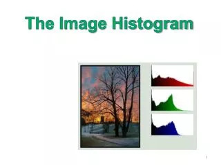
The Image Histogram • H(k) specifies the # of pixels with gray-value k • Let N be the number of pixels: • P(k) = H(k)/N defines the normalized histogram • defines the accumulated histogram Occurrence (# of pixels) Gray Level
Histogram Normalized Histogram Accumulated Histogram
Examples P(I) P(I) 1 • The image histogram does not fully represent the image 1 0.5 I I H(I) H(I) 0.1 0.1 I I Pixel permutation of the left image
P(I) 0.1 Original image I P(I) Decreasing contrast 0.1 I P(I) 0.1 Increasing average I
Image Statistics • The image mean: • Generally: • The image s.t.d. : 0.25 0.2 0.15 0.1 0.05 0 1 2 3 4 5 6 7 8 9 10 gray level
Image Entropy • The image entropy specifies the uncertainty in the image values. • Measures the averaged amount of information required to encode the image values. Entropy of a 2 values variable
An infrequent event provides more information than a frequent event • Entropy is a measure of histogram dispersion entropy=7.4635 entropy=0
Adaptive Histogram • In many cases histograms are needed for local areas in an image • Examples: • Pattern detection • adaptive enhancement • adaptive thresholding • tracking
Implementation: Integral Histogram • Integral histogram: H(x,y) represent the histogram of a window whose right-bottom corner is (x,y) • Construct by can order: H(x,y)= H(x,y-1)+H(x-1,y) – H(x-1,y-1) H(x-1,y-1) H(x,y-1) H(x,y) porkili 05 H(x-1,y)
Using integral histogram we can calculate local histograms of any window H(x1:x2,y1:y2) x (x2,y1) y (x1,y1) (x2,y2) (x1,y2) H(x1:x2,y1:y2) =H(x2,y2)+ H(x1,y1)-H(x1,y2)-H(x2,y1)
Histogram Usage • Digitizing parameters • Measuring image properties: • Average • Variance • Entropy • Contrast • Area (for a given gray-level range) • Threshold selection • Image distance • Image Enhancement • Histogram equalization • Histogram stretching • Histogram matching
Example: Auto-Focus • In some optical equipment (e.g. slide projectors) inappropriate lens position creates a blurred (“out-of-focus”) image • We would like to automatically adjust the lens • How can we measure the amount of blurring?
Image mean is not affected by blurring • Image s.t.d. (entropy) is decreased by blurring • Algorithm: Adjust lens according the changes in the histogram s.t.d.
Thresholding knew F(k) 255 kold 255 Threshold value
Threshold Selection Original Image Binary Image Threshold too low Threshold too high
Segmentation using Thresholding Original Histogram 50 75 Threshold = 75 Threshold = 50
Segmentation using Thresholding Original Histogram 21 Threshold = 21
Adaptive Thresholding • Thresholding is space variant. • How can we choose the the local threshold values?
Color Segmentation • Segmentation is based on color values. • Apply clustering in color space (e.g. k-means). • Segment each pixel to its closest cluster.
Histogram based image distance • Problem: Given two images A and B whose (normalized) histogram are PA and PB define the distance D(A,B) between the images. • Example Usage: • Tracking • Image retrieval • Registration • Detection • Many more ... Porkili 05
Option 1: Minkowski Distance • Problem: distance may not reflects the perceived dissimilarity: <
Option 2: Kullback-Leibler (KL) Distance • Measures the amount of added information needed to encode image A based on the histogram of image B. • Non-symmetric: DKL(A,B)DKL(B,A) • Suffers from the same drawback of the Minkowski distance.
Option 3: The Earth Mover Distance (EMD) • Suggested by Rubner & Tomasi 98 • Defines as the minimum amount of “work” needed to transform histogram HA towards HB • The term dij defines the “ground distance” between gray-levels i and j. • The term F={fij} is an admissible flow from HA(i) to HB(j) >
Option 3: The Earth Mover Distance (EMD) ≠ From: Pete Barnum
Option 3: The Earth Mover Distance (EMD) ≠ From: Pete Barnum
Option 3: The Earth Mover Distance (EMD) = From: Pete Barnum
Option 3: The Earth Mover Distance (EMD) (amount moved) = From: Pete Barnum
Option 3: The Earth Mover Distance (EMD) work=(amount moved) * (distance moved) = From: Pete Barnum
Option 3: The Earth Mover Distance (EMD) • Constraints: • Move earth only from A to B • After move PA will be equal to PB • Cannot send more “earth” than there is • Can be solved using Linear Programming • Can be applied in high dim. histograms (color).
Special case: EMD in 1D • Define CA and CB as the accumulated histograms of image A and B respectively: PA CA PB CB CA-CB
![[Image Similarity Based on Histogram]](https://cdn0.slideserve.com/1309335/image-similarity-based-on-histogram-dt.jpg)

![[Image Similarity Based on Histogram]](https://cdn5.slideserve.com/9279474/image-similarity-based-on-histogram-dt.jpg)