HISTOGRAM TRANSFORMATION IN IMAGE PROCESSING
HISTOGRAM TRANSFORMATION IN IMAGE PROCESSING. SHINTA P TEKNIK INFORMATIKA STMIK MDP 2013. Contents. Histogram Histogram transformation Histogram equalization Contrast streching Applications. Histogram. The (intensity or brightness) histogram shows how many

HISTOGRAM TRANSFORMATION IN IMAGE PROCESSING
E N D
Presentation Transcript
HISTOGRAM TRANSFORMATION IN IMAGE PROCESSING SHINTA P TEKNIK INFORMATIKA STMIK MDP 2013
Contents • Histogram • Histogram transformation • Histogram equalization • Contrast streching • Applications
Histogram The (intensity or brightness) histogram shows how many times a particular grey level (intensity) appears in an image. For example, 0 - black, 255 – white image histogram
Histogram (Cont) An image has low contrast when the complete range of possible values is not used. Inspection of the histogram shows this lack of contrast.
Histogram of color images RGB color can be converted to a gray scale value by Y = 0.299R + 0.587G + 0.114B Y: the grayscale component in the YIQ color space used in NTSC television. The weights reflect the eye's brightness sensitivity to the color primaries.
Histogram of color images (Cont) Histogram: individual histograms of red, green and blue Blue
Histogram of Color images (Cont) R B R G
Histogram of color images (Cont) or a 3-D histogram can be produced, with thethree axes representing the red, blue and green channels, and brightness at each point representing the pixel count
Histogram transformation sk rk grey values: Point operation T(rk) =sk T Properties of T: keeps the original range of grey values monoton increasing
Histogram Equalization (HE) Transforms the intensity values so that the histogram of the output image approximately matches the flat (uniform) histogram
Histogram equalization (Cont) As for the discrete case the following formula applies: k = 0,1,2,...,L-1 L: number of grey levels in image (e.g., 255) nj: number of times j-th grey level appears in image n: total number of pixels in the image ·(L-1) ?
Histogram Equalization (Cont) cumulative histogram
Histogram Equalization (Cont) histogram can be taken also on a part of the image
Histogram Projection (HP) Assigns equal display space to every occupied raw signal level, regardless of how many pixels are at that same level. In effect, the raw signal histogram is "projected" into a similar-looking display histogram.
Histogram projection (Cont) IR image HP HE
Histogram projection (Cont) occupied (used) grey level: there is at least one pixel with that grey level B(k): the fraction of occupied grey levels at or below grey level k B(k) rises from 0 to 1 in discrete uniform steps of 1/n, where n is the total number of occupied levels HP transformation: sk = 255 ·B(k).
Plateau equalization By clipping the histogram count at a saturation or plateauvalue, one can produce display allocations intermediate in character between those of HP and HE.
Plateau equalization (Cont) PE 50 HE
Plateau equalization (Cont) The PE algorithm computes the distribution not for the full image histogram but for the histogram clipped at a plateau (or saturation) value in the count. When that plateau value is set at 1, we generate B(k) and so perform HP; When it is set above the histogram peak, we generate F(k) and so perform HE. At intermediate values, we generate an intermediate distribution which we denote by P(k). PE transformation: sk = 255·P(k)
Histogram specification (HS) an image's histogram is transformed according to a desired function Transforming the intensity values so that the histogram of the output image approximately matches a specified histogram.
Histogram specification (Cont) histogram1 histogram2 S-1*T T S ?
Contrast streching (CS) By stretching the histogram we attempt to use the available full grey level range. The appropriate CS transformation : sk = 255·(rk-min)/(max-min)
Contrast streching (Cont) CS does not help here ? HE
Contrast streching (Cont) CS 1% - 99%
Contrast streching (Cont) HE CS 79, 136 CS Cutoff fraction: 0.8
Contrast streching (Cont) a more general CS: 0, if rk <plow sk = 255·(rk- plow)/(phigh - plow), otherwise 255, if rk >phigh
Applications CT lung studies Thresholding Normalization Normalization of MRI images Presentation of high dynamic images (IR, CT)
CT lung studies Yinpeng Jin HE taken in a part of the image
CT lung studies R.Rienmuller
Thresholding converting a greyscale image to a binary one for example, when the histogram is bi-modal threshold: 120
Thresholding (Cont) when the histogram is not bi-modal threshold: 80 threshold: 120
Normalization (Cont) When one wishes to compare two or more images on a specific basis, such as texture, it is common to first normalize their histograms to a "standard" histogram. This can be especially useful when the images have been acquired under different circumstances. Such a normalization is, for example, HE.
Normalization (Cont) Histogram matching takes into account the shape of the histogram of the original image and the one being matched.
Normalization of MRI images MRI intensities do not have a fixed meaning, not even within the same protocol for the same body region obtained on the same scanner for the same patient.
Normalization of MRI images (Cont) L. G. Nyúl, J. K. Udupa
Normalization of MRI images (Cont) A: Histograms of 10 FSE PD brain volume images of MS patients. B: The same histograms after scaling. C: The histograms after final standardization. L. G. Nyúl, J. K. Udupa A B C
m1 p1 p2 m2 m1 p1 p2 m2 Normalization of MRI images (Cont) bimodal unimodal • Method: transforming image histograms by landmark matching • Determine location of landmark i (example: mode, median, • various percentiles (quartiles, deciles)). • Map intensity of interest to standard scale for each volume image • linearly and determine the location ’s of i on standard scale.
Applications (Cont) A digitized high dynamic range image, such as an infrared (IR) image or a CAT scan image, spans a much larger range of levels than the typical values (0 - 255) available for monitor display. The function of a good display algorithm is to map these digitized raw signal levels into display values from 0 to 255 (black to white), preserving as much information as possible for the purposes of the human observer.
Applications (Cont) The HP algorithm is widely used by infrared (IR) camera manufacturers as a real-time automated image display. The PE algorithm is used in the B-52 IR navigation and targeting sensor.

![[Image Similarity Based on Histogram]](https://cdn0.slideserve.com/1309335/image-similarity-based-on-histogram-dt.jpg)


![[Image Similarity Based on Histogram]](https://cdn5.slideserve.com/9279474/image-similarity-based-on-histogram-dt.jpg)