Image Transformation
Image Transformation. Spatial domain (SD) and Frequency domain (FD) Fourier Transform: SD FD Hough Transform: SD SD Wavelet Transform: SD FD + SD Geometric Transform: spatial distortion correction, image warping, image interpolation. Frequency domain. Fourier transform:
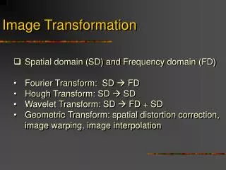

Image Transformation
E N D
Presentation Transcript
Image Transformation • Spatial domain (SD) and Frequency domain (FD) • Fourier Transform: SD FD • Hough Transform: SD SD • Wavelet Transform: SD FD + SD • Geometric Transform: spatial distortion correction, image warping, image interpolation
Frequency domain • Fourier transform: • -- periodic function can be represented as a weighted sum of sines and cosines • 1-D: • F(u) – frequency components • u – frequency • Domain on “u” – frequency domain
Frequency domain (cont’d) • 2D Fourier transform: • -- Forward transform: • -- Inverse transform: • Where x, y are in the range (–infinity, +infinity) • u, v are in the range (–infinity, +infinity)
Frequency domain (cont’d) • Discrete Fourier transform (DFT) • -- Forward transform: • -- Inverse transform: • Where x=0,1, …, M-1 • u=0,1, …, M-1
Frequency domain (cont’d) • Discrete Fourier transform (DFT) • Applying Euler’s formula: • We obtain:
Frequency domain (cont’d) • Discrete Fourier transform (DFT) • Polar coordinate representation: • Frequency u=0: flat uniform signal has zero frequency. • |F(0)| = (A*k)/M • Where: k points out of M points have value A (non-zero) in spatial domain f(x) A x k M
Frequency domain (cont’d) M u F(0,0) • 2D DFT • Image size: M * N • -- Forward transform: • -- Inverse transform: • Where x, y – spatial variable • u, v – frequency variable N v
Filtering in frequency domain -- Image smoothing -- Image sharpening (enhancement) F(u,v) --- > H(u,v) --- > G(u,v) H(u,v) – filter transfer function -- increase or pass certain band of frequencies -- depress other bands of frequencies
Filtering Operations • Computation • There is correspondence between the filtering in SD and FD • Convolution definition (denote as )
Filtering Operations • SD and FD
Filtering Operations • Gaussian Filter • Note: large sigma broad profile H(u) • narrow profile of h(x)
Basis or kernel of transformation • Transform basis • Consider an image f(x,y) of size N*N,whose discrete transform is T(u,v) • x,y,u,v = 0, 1, …, N-1 • T(u,v) – transform coefficient
Basis or kernel of transformation • Transform basis (cont’d) • Example: Walsh-Hadamard transform • g(x,y,u,v) = 1/N * (-1)B • h(x,y,u,v) = 1/N * (-1)B • Where: • B= SUM_{i=0}^{m-1} mod2(bi(x)pi(u) + bi(y)pi(v)) • N = 2m • bi(x) – ith bit in the binary representation of x
Basis or kernel of transformation • Transform basis (cont’d) • Example: Walsh-Hadamard transform • B= SUM_{i=0}^{m-1} mod2(bi(x)pi(u) + bi(y)pi(v)) • p0(u) = bm-1(u) • p1(u) = bm-1(u) + bm-2(u) • : • : • pm-1(u) = b1(u) + b0(u)
Basis or kernel of transformation • Transform basis (cont’d) • Example: Discrete cosine transform (DCT) • Kernel: • where: a(u) = sqrt(1/N) when u=0 • = sqrt(2/N) when u=1,2,…, N-1
Basis or kernel of transformation • Transform basis (cont’d) Example: 2-D DCT and IDCT • DCT: • IDCT: • where: Note: u,v =0 (DC, low frequency) u,v increase (AC, high frequency)
Basis or kernel of transformation • Transform basis (cont’d) Example: 2-D DCT and IDCT • DCT: • IDCT: 2D DCT Frequencies (8*8) (64 basis functions)
Basis or kernel of transformation • Transform basis (cont’d) Example: Principal component analysis (PCA) (or called Karhunen-Loeve (K-L) transform) (or Hotelling transform) -- statistics-based transform (kernel is not fixed) -- application: data compression, rotation, etc.
Basis or kernel of transformation • PCA (cont’d) • Mean vector and covariance matrices • There are n images which have same contents. • Suppose each image has k pixels. • A pixel vector Xi at position i is composed of n components. • Xi =[xi1, xi2, …, xin] i 1 2 3 … n
Basis or kernel of transformation • PCA (cont’d) • Mean vector • Covariance matrices • T – transpose
Basis or kernel of transformation • PCA (cont’d) • Cx is a real symmetric matrix. • There must be an orthogonal matrix A, such that Cx can be transformed to a diagonal matrix Cy • A Cx AT = Cy • A is an orthogonal matrix which consists of n orthogonal vectors • A-1 = AT
Basis or kernel of transformation • PCA (cont’d) • Because Cx is a real symmetric matrix, it is possible to find a set of n orthogonal eigenvectors {ei} and the corresponding eigenvalues {i}, i=1,2,…, n. • Definition of eigenvectors and eigenvalues of n*n matrix C • Cx ei = i ei, i=1,2,…, n. • where 1 >2 …>n • eiT ej = 1 if i=j • = 0 if i j
Basis or kernel of transformation • PCA (cont’d) • Cy = A Cx AT
Basis or kernel of transformation • PCA (cont’d) • Forward transform: map the vector x into vector y • Inverse transform: • Cy and Cx have same eigenvectors and same eigenvalues
Basis or kernel of transformation • PCA (cont’d) • Applications: -- compression • We can select most significant eigenvectors to approximate the A
Basis or kernel of transformation • PCA (cont’d) • Applications: -- compression (cont’d) • The mean square error between vector X and vector Xk is SUM_{j=k+1}^{n} j
Basis or kernel of transformation • PCA (cont’d) • Applications: -- compression (cont’d) • Property • (1) mean square error is minimized after the transform • (2) Kernel “A” is not separable (“image-dependant”) • Example: • (1) Apply PCA to 6 images (textbook page 679-682) • As a result, 6 images can be represented by • “ 2 transformed images (e.g. y coefficients) • + transform matrix A (e.g., first two rows) • + mean vector”
Basis or kernel of transformation • PCA (cont’d) • Example • -- Eigen-face • -- Object rotation (coordinate transform)
Basis or kernel of transformation • PCA (cont’d) • Comparison • -- PCA is image-adaptive compression which has optimal performance -- DCT is much closer to PCA PCA Log(e2) DCT DFT WHT k number of coefficients Compression performance comparison
Hough Transform • Purpose • -- Detection of specific structure relationships between pixels in an image • -- Spatial domain to spatial domain transformation • -- Example: • Given a set of points in an image, we want to find subsets of these points that lie on straight lines or on a circle
Hough Transform (cont’d) • Parameter space • Spatial line representation: • -- Slope-intercept form: • yi = axi +b • -- ab-plane representation (parameter space) • b = -axi + yi
Hough Transform (cont’d) • Hough transform for straight line detection b’ b y b=-axi + yi xi, yi a’ b=-axj + yj xj, yj a x xy plane ab plane
Hough Transform (cont’d) • Hough transform for straight line detection (cont’d) -- One line in parameter space corresponds to a point in image space -- All points on a line (y=ax+b) will have lines in parameter space that intersect at (a,b).
Hough Transform (cont’d) • Hough transform for straight line detection (cont’d) bmin 0 bmax b amin : … … 0 : amax a Discrete ab plane
Hough Transform (cont’d) • Discrete parameter space -- Subdividing the parameter space into accumulator cells, where (amax, amin) and (bmax, bmin) are the expected ranges of slope and intercept values. -- The cell at coordinates (i, j), with accumulator value A(i,j), corresponds to the square associated with parameter space coordinates (ai, bj).
Hough Transform (cont’d) • Line detection in discrete parameter space -- Initially, all cells are set to zero A(i,j)=0 -- Calculate (ai, bj) for each (xk, yk); If the line passes through cell (i,j) then A(i,j)= A(i,j) +1 -- The cell with maximum accumulator value indicates a line in the image plane, which contains the most points (i.e., collinear points)
Hough Transform (cont’d) • Problem in Line detection Vertical line can not be represented in the slope-intercept form y=ax+b (a ) • -plane representation xcos() + ysin() = - each line in image plane is determined by angle and distance . - (i,i) in parameter space is in cell (i,j), which is associated with an accumulator A(i,j) - [-90°, 90°], measured with respect to the x axis
Hough Transform (cont’d) • -plane representation xcos() + ysin() = min max 0 min : y … … 0 : max x Discrete -plane
Hough Transform (cont’d) • Hough transform for circle detection -- Hough transforms applicable to any function of the form g(x,c)=0, where x is a vector of coordinates and c is a vector of coefficients -- Example: Points on the circle (x-c1)2 + (y-c2)2 =c32 can be detected by 3D parameter space (c1, c2, c3)
Hough Transform (cont’d) • Hough transform for circle detection -- Cube-like cells and accumulators A(i,j,k). -- The complexity increases if the number of coordinates and coefficients increases. c3 c2 c1