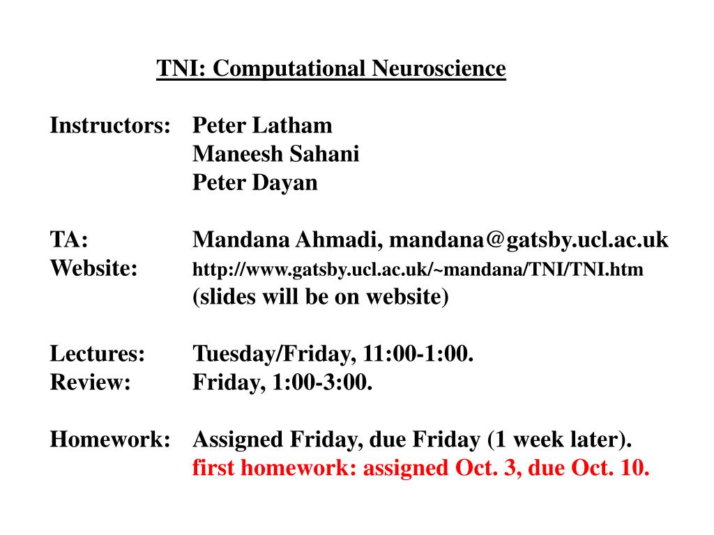
1. TNI: Computational Neuroscience Instructors: Peter Latham Maneesh Sahani Peter Dayan TA: Mandana Ahmadi, mandana@gatsby.ucl.ac.uk Website: http://www.gatsby.ucl.ac.uk/~mandana/TNI/TNI.htm (slides will be on website) Lectures: Tuesday/Friday, 11:00-1:00. Review: Friday, 1:00-3:00. Homework: Assigned Friday, due Friday (1 week later). first homework: assigned Oct. 3, due Oct. 10.

2. What is computational neuroscience? Our goal: figure out how the brain works.

3. There are about 10 billion cubes of this size in your brain! 10 microns

4. How do we go about making sense of this mess? David Marr (1945-1980) proposed three levels of analysis: 1. the problem (computational level) 2. the strategy (algorithmic level) 3. how it’s actually done by networks of neurons (implementational level)

5. Example #1: memory. the problem: recall events, typically based on partial information.

6. r3 r2 r1 activity space Example #1: memory. the problem: recall events, typically based on partial information. associative or content-addressable memory. an algorithm: dynamical systems with fixed points.

7. Example #1: memory. the problem: recall events, typically based on partial information. associative or content-addressable memory. an algorithm: dynamical systems with fixed points. neural implementation: Hopfield networks. xi = sign(∑j Jij xj)

8. Example #2: vision. the problem (Marr): 2-D image on retina → 3-D reconstruction of a visual scene.

9. Example #2: vision. the problem (modern version): 2-D image on retina → recover the latent variables. house sun tree bad artist

10. Example #2: vision. the problem (modern version): 2-D image on retina → reconstruction of latent variables. an algorithm: graphical models. x1 x2 x3 latent variables r1 r2 r3 r4 low level representation

11. Example #2: vision. the problem (modern version): 2-D image on retina → reconstruction of latent variables. an algorithm: graphical models. x1 x2 x3 latent variables inference r1 r2 r3 r4 low level representation

12. Example #2: vision. the problem (modern version): 2-D image on retina → reconstruction of latent variables. an algorithm: graphical models. implementation in networks of neurons: no clue.

13. Comment #1: the problem: the algorithm: neural implementation:

14. Comment #1: the problem: easier the algorithm: harder neural implementation: harder often ignored!!!

15. Comment #1: the problem: easier the algorithm: harder neural implementation: harder A common approach: Experimental observation → model Usually very underconstrained!!!!

16. Comment #1: the problem: easier the algorithm: harder neural implementation: harder Example i: CPGs (central pattern generators) rate rate Too easy!!!

17. Comment #1: the problem: easier the algorithm: harder neural implementation: harder Example ii: single cell modeling CdV/dt = -gL(V – VL) – n4(V – VNa) … dn/dt = … … lots and lots of parameters … which ones should you use?

18. Comment #1: the problem: easier the algorithm: harder neural implementation: harder Example iii: network modeling lots and lots of parameters × thousands

19. r3 x1 x2 x3 r2 r1 r2 r3 r4 r1 activity space Comment #2: the problem: easier the algorithm: harder neural implementation: harder You need to know a lot of math!!!!!

20. Comment #3: the problem: easier the algorithm: harder neural implementation: harder This is a good goal, but it’s hard to do in practice. Our actual bread and butter: 1. Explaining observations (mathematically) 2. Using sophisticated analysis to design simple experiments that test hypotheses.

21. dendrites soma axon +40 mV 1 ms voltage -50 mV 100 ms time A classic example: Hodgkin and Huxley.

22. A classic example: Hodgkin and Huxley. CdV/dt = –gL(V-VL) – gNam3h(V-VNa) – … dm/dt = … …

23. Comment #4: the problem: easier the algorithm: harder neural implementation: harder some algorithms are easy to implement on a computer but hard in a brain, and vice-versa. we should be looking for the vice-versa ones. it can be hard to tell which is which. these are linked!!!

24. Basic facts about the brain

25. Your brain

26. Your cortex unfolded neocortex (cognition) 6 layers ~30 cm ~0.5 cm subcortical structures (emotions, reward, homeostasis, much much more)

27. Your cortex unfolded 1 cubic millimeter, ~3*10-5 oz

28. 1 mm3 of cortex: 50,000 neurons 10000 connections/neuron (=> 500 million connections) 4 km of axons

29. 1 mm3 of cortex: 50,000 neurons 10000 connections/neuron (=> 500 million connections) 4 km of axons 1 mm2 of a CPU: 1 million transistors 2 connections/transistor (=> 2 million connections) .002 km of wire

30. 1 mm3 of cortex: 50,000 neurons 10000 connections/neuron (=> 500 million connections) 4 km of axons whole brain (2 kg): 1011 neurons 1015 connections 8 million km of axons 1 mm2 of a CPU: 1 million transistors 2 connections/transistor (=> 2 million connections) .002 km of wire whole CPU: 109 transistors 2*109 connections 2 km of wire

31. 1 mm3 of cortex: 50,000 neurons 10000 connections/neuron (=> 500 million connections) 4 km of axons whole brain (2 kg): 1011 neurons 1015 connections 8 million km of axons 1 mm2 of a CPU: 1 million transistors 2 connections/transistor (=> 2 million connections) .002 km of wire whole CPU: 109 transistors 2*109 connections 2 km of wire

32. dendrites (input) soma (spike generation) axon (output) +40 mV 1 ms voltage -50 mV 100 ms time

34. synapse current flow

35. synapse current flow

36. +40 mV voltage -50 mV 100 ms time

37. neuron i neuron j neuron j emits a spike: EPSP V on neuron i t 10 ms

38. neuron i neuron j neuron j emits a spike: IPSP V on neuron i t 10 ms

39. neuron i neuron j neuron j emits a spike: IPSP V on neuron i t amplitude = wij 10 ms

40. neuron i neuron j neuron j emits a spike: changes with learning IPSP V on neuron i t amplitude = wij 10 ms

41. synapse current flow

42. A bigger picture view of the brain

43. x latent variables peripheral spikes r sensory processing ^ r “direct” code for latent variables cognition memory action selection brain ^ r' “direct” code for motor actions motor processing r' peripheral spikes x' motor actions

44. r

45. r

46. r

47. r

48. you are the cutest stick figure ever! r

49. you are the cutest stick figure ever! r

50. x latent variables peripheral spikes r sensory processing ^ r “direct” code for latent variables cognition memory action selection brain ^ r' “direct” code for motor actions motor processing r' peripheral spikes x' motor actions