Download
1 / 1
10 likes | 168 Vues
.55. False negatives (lowest-scoring). False positives (highest-scoring). True positives (highest-scoring). .22. .46. .83. Crystal. .60. .04. Crystal + Phase Sep. .16. .62. .98. .52. Crystal + Precip. Precip. Precip + Skin. Precip + Phase Sep. Phase Sep. + Skin.

E N D
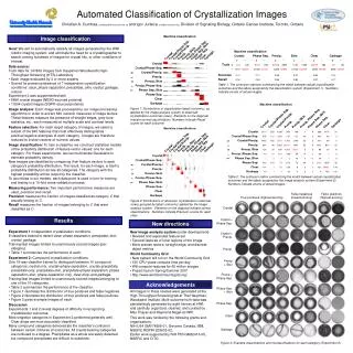
.55 False negatives (lowest-scoring) False positives (highest-scoring) True positives (highest-scoring) .22 .46 .83 Crystal .60 .04 Crystal + Phase Sep. .16 .62 .98 .52 Crystal + Precip. Precip. Precip + Skin Precip + Phase Sep. Phase Sep. + Skin Phase Sep. Table 1: The confusion matrices summarizing the match between actual crystallization outcomes and the labels assigned by the classification system (Experiment 1). Numbers indicate counts of actual images. Clear Garbage Figure 1: Distributions of classification labels (columns), as applied by the image analysis system to observed crystallization outcomes (rows). Elements on the diagonal indicate correct classifications. Numbers indicate Recall scores for each outcome. Figure 2: Distributions of observed crystallization outcomes (rows) grouped by labels (columns) applied by the image analysis system. Elements on the diagonal indicate correct classifications. Numbers indicate Precision scores for each class. Table 2: The confusion matrix summarizing the match between actual crystallization outcomes and the labels assigned by the image analysis system (Experiment 2). Numbers indicate counts of actual images. Figure 3: Example classifications and misclassifications for each category (Experiment 2). Automated Classification of Crystallization Images Christian A. Cumbaa ccumbaa@uhnres.utoronto.ca and Igor Jurisica juris@cs.utoronto.ca, Division of Signaling Biology, Ontario Cancer Institute, Toronto, Ontario Image classification • Goal: We aim to automatically classify all images generated by the HWI robotic imaging system, and eliminate the need for a crystallographer to search among hundreds of images for crystal hits, or other conditions of interest. • Data source: • Truth data for 147456 images from Hauptman Woodward's High-Throughput Screening (HTS) Laboratory • Each image evaluated by 3 or more experts • Scored for presence/absence of 7 independent crystallization conditions: clear, phase separation, precipitate, skin, crystal, garbage, unsure • Experiment 2 was supplemented with • 6456 crystal images (NESG-sourced proteins) • 11504 crystal images (SGPP-sourced proteins) • Image analysis: Each image was processed by our image processing algorithms in order to extract 840 numeric measures of image texture. These features measure the presence of straight edges, grey-tone statistics, etc., each measured at multiple scale and contrast levels. • Feature selection: For each target category of images, we select a subset of the 840 features that most effectively distinguishes positive/negative examples of each category. Images are therefore reduced to a short vectors of numeric values. • Image classification: To train a classifier, we construct statistical models of the probability distribution of feature-vector values: one for each category. For these experiments, we use multivariate Gaussians to estimate probability density. • New images are classified by comparing their feature vectors to each category's probability distribution. The result, for each image, is itself a probability distribution across all categories. The category with the highest probability will be output by the classifier. • To avoid bias in our models, each data point is used in turn for training and testing in a 10-fold cross-validation process. • Measuring performance: Two important performance measures are used, precision and recall. • Precision measures the fraction of images classified as category C that actually belong to C. • Recall measures the fraction of images belonging to C that were classified as C. .59 .38 .49 .86 .62 .13 .38 .61 .89 .48 Results New directions • Experiment 1: Independent crystallization conditions. • 6 classifiers trained to detect clear, phase separation, precipitate, skin, crystal, garbage. • Training/test images limited to unanimously-scored images (per-category). • Table 1 summarizes the performance of each. • Experiment 2: Compound crystallization conditions. • One 10-way classifier trained to distinguish between 10 compound categories: crystal only, crystal+phase separation, crystal+precipitate, precipitate only, precipitate+skin, precipitate+phase separation, phase separation+skin, phase separation only, clear drop, and garbage. • Training/test images limited to unanimously-scored images belonging to one of the 10 categories. • Table 2 summarizes the performance of the classifier. • Figure 1 illustrates the distribution of true positives and false negatives. • Figure 2 illustrates the distribution of true positives and false positives. • Figure 3 gives example images of each. • Discussion • Experiments 1 and 2 reveal degrees of difficulty in recognizing crystallization outcomes. • Most singleton categories in Experiment 2 performed generally well. Clear drops are most accurately classified. • Many compound categories demonstrate the classifier's confusion between certain mixtures of outcomes. All crystal-bearing categories are confused to a degree. Precipitates as a whole are easily detected, but compound precipitates are difficult to subdivide. • New image analysis system (under development) • Revised and expanded feature set • Textural features of local regions of the image • More precise texture, straight edge, and discrete object metrics • World Community Grid • New system will run on the World Community Grid • 150 CPU-years compute time per day • Will compute features for 60 million images • Project launch Spring/Summer 2007 • http://www.worldcommunitygrid.org/ Acknowledgements All images in these studies were generated at the High-Throughput Screening lab at The Hauptman-Woodward Institute. Multi-outcome truth data was painstakingly generated by eight heroes at HWI, and carefully organized, cleaned, and curated by Max Thayer and Raymond Nagel at HWI. This work was funded by the following grants and organizations: NIH U54 GM074899-01, Genome Canada, IBM, NSERC RGPIN 203833-02. Earlier work supported by NIH P50 GM62413-05, NSERC and CITO.