Download

1 / 69
690 likes | 710 Vues
Join the workshop to learn about population dynamics in fisheries, including mortality rates, growth functions, and stock-recruitment relationships using R software. Analyze Pygmy Whitefish data from Lake Superior and explore age-length relationships.

E N D
R for Fisheries Population Dynamcs Western Division of AFS Student Colloquium 15 November 2017
Who I Am? Derek Professor of Mathematical Sciences and Natural Resources at Northland College Ph.D. in Fisheries with minor in Statistics from University of Minnesota
Who I Am? Author:Introductory Fisheries Analyses with R Maintainer:fishR website Author & Maintainer: FSA and FSAdata R packages
Workshop Objectives • Introduction to typical population dynamic rate functions, including • mortality rates • growth functions • stock-recruitment relationships • Methods to compare parameter estimates • Additional topics (depending on time) • Weight-length relationships (and comparisons) • Reproducible research documents
Workshop Data I Pygmy Whitefish (Prosopiumcoulterii)
Workshop Data I • Pygmy Whitefish (Prosopiumcoulterii) • Sampled with a bottom trawl from 28 locations throughout Lake Superior • TL (mm) and region recorded for all fish • Weight (g) and age from thin-sectioned otoliths recorded for a length-stratified subsample • Modified from “Age, Growth, and Size of Lake Superior Pygmy Whitefish” (Stewart et al. 2016)
Pygmy Whitefish Script Initial Preparations Initial Data Wrangling (and Quick Summaries)
Age-Length Key – Concept Full Sample len age 32 NA 27 NA 36 NA 21 1 22 NA 30 NA 31 NA ... ... len age 22 1 24 NA 26 NA 27 2 30 1 32 NA 34 2 ... ... Age Sample len age 22 1 27 2 30 1 34 2 • 21 1 ... ...
Age-Length Key – Development • Use 10-cm intervals for length categories • Make raw frequency table • Age • LCat 1 2 3 • 20 • 30 • 40 • 50 • Convert to row-proportions table • Age • LCat 1 2 3 • 20 • 30 • 40 • 50 LCat 20 20 20 20 30 30 30 30 40 40 40 40 50 50 50 50 2 2 0 1 2 1 1 1 2 0 2 2 0.50 0.50 0.00 0.25 0.50 0.25 0.25 0.25 0.50 0.00 0.50 0.50 Age Sample len age 22 1 24 1 26 2 27 2 30 1 32 2 34 2 39 3 40 1 44 2 46 3 49 3 52 2 53 2 55 3 56 3
Pygmy Whitefish Script Create Age-Length Key Do assignment
Age-Length Key – Concept Full Sample Modified Full Sample len age 32 NA 27 NA 36 NA 21 1 22 NA 30 NA 31 NA ... ... len age 32 3 272 362 21 1 22 1 30 1 31 2 ... ... len age 22 1 24 NA 26 NA 27 2 30 1 32 NA 34 2 ... ... len age 22 1 24 1 26 2 27 2 30 1 32 2 34 2 ... ... Length Sample Modified Length Age Sample len age 24 NA 26 NA 32 NA 32 NA 27 NA 36 NA 22 NA 30 NA 31 NA ... ... len age 24 1 26 2 32 3 32 2 27 2 36 2 22 1 30 1 31 2 ... ... ALK len age 22 1 27 2 30 1 34 2 • 21 1 ... ...
Age-Length Key – Assign Ages • Create same length categories • Construct length distribution • LCat 20 30 40 50 • Freq 4 3 5 2 LCat 20 20 20 20 30 30 30 40 40 40 40 40 50 50 Length Sample len age 23 25 26 28 32 33 36 40 43 44 48 49 51 54
Age-Length Key – Assign Ages • Length distribution (as a reminder) • LCat 20 30 40 50 • Freq 4 3 5 2 • Age-Length Key (as a reminder) • LCat 1 2 3 • 20 0.50 0.50 0.00 • 30 0.25 0.50 0.25 • 40 0.25 0.25 0.50 • 50 0.00 0.50 0.50 • Identify number in each length category to be assigned each age • 20-cm 4*0.5 = 2 age-1 • 4*0.5 = 2 age-2 • 4*0 = 0 age-3 • Randomly assign these ages LCat 20 20 20 20 30 30 30 40 40 40 40 40 50 50 1 2 2 1 Length Sample len age 23 25 26 28 32 33 36 40 43 44 48 49 51 54
Age-Length Key – Assign Ages • Length distribution (as a reminder) • LCat 20 30 40 50 • Freq 4 3 5 2 • Age-Length Key (as a reminder) • LCat 1 2 3 • 20 0.50 0.50 0.00 • 30 0.25 0.50 0.25 • 40 0.25 0.25 0.50 • 50 0.00 0.50 0.50 • Identify number in each length category to be assigned each age • 30-cm 3*0.25 = 0.75 age-1 • 3*0.5 = 1.5 age-2 • 3*0.25 = 0.75 age-3 • What to do now? LCat 20 20 20 20 30 30 30 40 40 40 40 40 50 50 1 2 2 1 Length Sample len age 23 25 26 28 32 33 36 40 43 44 48 49 51 54
Age-Length Key – Fractionation • Round all values down to integers. • 30-cm 3*0.25 = 0.75 = 0 age-1 • 3*0.5 = 1.5= 1 age-2 • 3*0.25 = 0.75= 0 age-3 • For remaining two fish ... • Choose two ages such that age-1 has a 25%, age-2 has a 50%, and age-3 has a 25% chance of being selected. • e.g., 2, 1 were chosen • Thus, assign 1 age-1, 2 age-2, & 0age-3
Age-Length Key – Assign Ages • Length distribution (as a reminder) • LCat 20 30 40 50 • Freq 4 3 5 2 • Age-Length Key (as a reminder) • LCat 1 2 3 • 20 0.50 0.50 0.00 • 30 0.25 0.50 0.25 • 40 0.25 0.25 0.50 • 50 0.00 0.50 0.50 • Identify number in each length category to be assigned each age • 30-cm 3*0.25 = 0.75 age-1 • 3*0.5 = 1.5 age-2 • 3*0.25 = 0.75 age-3 • Randomly assign these ages LCat 20 20 20 20 30 30 30 40 40 40 40 40 50 50 1 2 2 1 2 1 2 1 2 0 Length Sample len age 23 25 26 28 32 33 36 40 43 44 48 49 51 54
Age-Length Key – Assign Ages • Length distribution (as a reminder) • LCat 20 30 40 50 • Freq 4 3 5 2 • Age-Length Key (as a reminder) • LCat 1 2 3 • 20 0.50 0.50 0.00 • 30 0.25 0.50 0.25 • 40 0.25 0.25 0.50 • 50 0.00 0.50 0.50 • Identify number in each length category to be assigned each age • 40-cm 5*0.25 = 1.25 = 1 age-1 • 5*0.25 = 1.25 = 1 age-2 • 5*0.5 = 2.5 = 2 age-3 • Extra fish was chosen to be age-3 • Randomly assign these ages LCat 20 20 20 20 30 30 30 40 40 40 40 40 50 50 1 2 2 1 2 1 2 3 1 2 1 3 1 3 3 Length Sample len age 23 25 26 28 32 33 36 40 43 44 48 49 51 54
Pygmy Whitefish Script Apply Age-Length Key Do assignment
Catch-at-Age Data • Follow 2010 cohort (i.e., year-class) assuming … • 10,000 fish hatched • sampled immediately with 2 units of effort and 1% catchability • 20% annual mortality Capture Year Age2010 2011 2012 2013 2014 2015 2016 2017 0 1 2 3 4 5 200 160 128 102 82 66
Catch-at-Age Data • Follow 2010 cohort (i.e., year-class) • Follow 2011cohort (i.e., year-class) assuming … • same as for 2010 cohort Capture Year Age2010 2011 2012 2013 2014 2015 2016 2017 0 1 2 3 4 5 200 200 160 160 128 128 102 102 82 82 66 66
Catch-at-Age Data • Follow 2010 cohort (i.e., year-class) • Follow 2011cohort (i.e., year-class • Remaining cohorts assuming the same Capture Year Age2010 2011 2012 2013 2014 2015 2016 2017 0 1 2 3 4 5 200 200 200 200 200 200 200 200 160 160 160 160 160 160 160 160 128 128 128 128 128 128 128 128 102 102 102 102 102 102 102 102 82 82 82 82 82 82 82 82 66 66 66 66 66 66 66 66
Catch-at-Age Data • Under the assumptions of • Constant recruitment • Constant mortality (between ages and years) • Constant catchability (between ages and years) • Longitudinal = cross-sectional catch-curve Capture Year Age2010 2011 2012 2013 2014 2015 2016 2017 0 1 2 3 4 5 200 200 200 200 200 200 200 200 160 160 160 160 160 160 160 160 128 128 128 128 128 128 128 128 102 102 102 102 102 102 102 102 82 82 82 82 82 82 82 82 66 66 66 66 66 66 66 66
Catch Curve Model • Note that • Ct= qEtNt and thus CPEt= qNt • Nt= N0(1-A)t • Nt= N0e-Zt • Substituting Nt = N0e-Zt into CPEt= qNt gives … CPEt= qN0e-Zt
Catch Curve Model • CPEt= qN0e-Zt • Can this be linearized? 200 160 CPE 120 80 0 1 2 3 4 5 Age / Time
4.0 3.5 3.0 2.5 log(CPE) 2.0 1.5 1.0 0.5 0 2 4 6 8 10 Age / Time Catch Curve Model -Z 1 -Z 1 Descending Asc Dome Transformed model: log(CPEt) = log(qN0)-Zt
Mortality Estimates • Z • Instantaneous total mortality rate • Annual decline in natural log of CPE • Uninterpretable • A • A=1-e-Z • Total annual mortality rate • Proportional decline in CPE • Easily interpretable
Catch Curve Decisions • Descending limb • Include age with peak catch • Use all ages where Ct>0 • though some argue for various right truncation rules • Weighted regression • Reduced effect of ages with low CPE • Demonstrated with R script • Chapman-Robson method • Generally preferred over regression method • Demonstrated in R script
Pygmy Whitefish Script Estimate Mortality Rates Do assignment
Comparing Mortality Rates • If catch curve slopes differ, then Z differs. • i.e., mortality rates differ. • Test for different slopes using dummy variable regression (aka indicator variable regression or ANCOVA).
Dummy/Indicator Variables • Numerical representation of a dichotomous factor variable • Indicator variable called countryUSA • countryUSA= 1if from USA • countryUSA= 0otherwise (i.e., from CANADA) • Named after “1” group • “0” group does not have characteristic • called the “reference” group
Interaction Variables • The product of two (or more) explanatory variables • Used to determine if the effect of one explanatory variable on the response variable is influenced by the value of another explanatory variable • Catch curve example • Interaction between ageand countryUSA • Is the effect of age on logfreq affected by country?
Ultimate Full Model • For catch curve example … • mlogfreq = a + bage + d1countryUSA + g1countryUSA*age • Order of explanatory variables: • Quantitative covariate • Individual indicator variables • Interaction between indicators and covariate • Coefficients are … • ais an intercept • b is on the covariate • di are on the indicator variables • gi are on the interaction variables
Submodels mlogfreq = a + bage + d1countryUSA + g1countryUSA*age • Reductions of the ultimate full model • represent each group in data • What happens when countryUSA = 0? • mlogfreq = a + bage • What happens when countryUSA = 1? • mlogfreq = a + bage + d1+ g1age = (a+d1) + (b+ g1)age
Comparing Mortality Rates not USA: mlogfreq = a + bage USA: mlogfreq = (a+d1) + (b+g1)age If catch curve slopes differ, then Z differs Test if the interaction variable is significant or not (i.e., is g1=0).
Pygmy Whitefish Script Compare Mortality Rates
Length-At-Age Data TL Age Species 24 6 Rainbow 26 8 Rainbow 23 5 Rainbow 25 5 Rainbow 24 4 Rainbow 24 5 Rainbow 23 4 Rainbow 25 5 Rainbow 20 4 Rainbow 23 4 Rainbow 26 6 Rainbow 29 10 Rainbow 20 4 Rainbow 29 8 Rainbow 24 6 Rainbow 26 6 Rainbow 23 5 Rainbow 24 4 Rainbow
Length-At-Age Models • Purposes • Summarize growth with few parameters. • Compare growth parameters among populations. • Use results in key fisheries models, such as Beverton-Holt yield models. • Main models • von Bertalanffy • Gompertz • Logistic • Richards
Von Bertalanffy – Typical • L∞ = asymptotic mean length • to = time when mean length is 0 (artifact)
Von Bertalanffy – Typical • L∞ = asymptotic mean length • to = time when mean length is 0 (artifact) • K= Brody “growth” coefficient • Controls “curvature” of the model • Rate at which E[L|t] approaches L∞ • log(2)/K is “half-life”
Non-Linear Modeling • However, no closed-form solution • Algorithms require starting values • Iteratively search for minimum RSS VBGF is non-linear, in shape and parameters Non-linear least-squares minimizes RSS
Non-Linear Modeling • Sampling distributions of parameter estimates tend NOT to be normally distributed. • Alternative CI #1 – Profile Likelihood Method • Use c2 and shape of likelihood function
Non-Linear Modeling • Sampling distributions of parameter estimates tend NOT to be normally distributed. • Alternative CI #2 – Bootstrapping • Construct a random sample (with replacement) of n “cases" of observed data. • Extract parameters from model fit to this (re)sample. • Repeat first two steps B times. • 95% CI is values of ordered parameter estimates with 2.5% of values lesser and 2.5% of values greater.
Von Bertalanffy – Typical For a thorough description see Ogle, D.H., T.O. Brenden, and J.L. McCormick. 2018. Growth Estimation: Growth Models and Statistical Inference. In Quist, M.C. and D. Isermann, editors. Age and Growth of Fishes: Principles and Techniques. American Fisheries Society. • Common Problems • Misinterpreted meanings • Difficulty modeling L∞ • Few old fish • Difficulty modeling K • Few young fish • Model won’t converge, Poor parameter estimates • Much variability in length at each age • Highly correlated parameters • “Scale” of L∞ much different than K or to • Type of error structure (additive or multiplicative)
Pygmy Whitefish Script Fit Growth Model Do assignment
Steps in Comparison • Fit {L∞,K,t0} and assess assumptions • Examine Script • Compare {L∞,K,t0} to {Ω} • Non-significant (p>a) no parameters differ between groups; Stop. • Significant (p<a) some parameter(s) differ between groups; Continue.
Model Comparisons • Extra Sum-of-Squares Test • “Is RSS significantly reduced?” • F-test • Likelihood Ratio Test • “Is likelihood significantly increased?” • “Is negative log likelihood significantly decreased?” • Chi-square test • Functionally equivalent for large n. • Examine Script
Steps in Comparison * • Compare {L∞,K}, {L∞,t0}, and {K,t0} to {L∞,K,t0} • Non-significant (p>a) the common parameter does not differ between groups. • Significant (p<a) the common parameter differs between groups. • All significant all parameters differ between groups; Stop. • Some non-significant choose model with lowest RSS, highest likelihood, or lowest negative log-likelihood as most parsimonious; Continue. • Examine Script