Download
1 / 69
690 likes | 748 Vues
Learn about aggregate output and income in macroeconomics and how spending behavior influences the economy. Explore consumption, saving, investment, and planned aggregate expenditure to understand economic equilibrium.

E N D
Aggregate Output andAggregate Income (Y) • Aggregate output is the total quantity of goods and services produced (or supplied) in an economy in a given period. • Aggregate income is the total income received by all factors of production in a given period.
Aggregate Output andAggregate Income (Y) • Aggregate output (income) (Y) is a combined term used to remind you of the exact equality between aggregate output and aggregate income. • When we talk about output (Y), we mean real output, or the quantities of goods and services produced, not the dollars in circulation.
Explaining Spending Behavior • All income is either spent on consumption or saved in an economy in which there are no taxes. Saving / Aggregate Income - Consumption
Household Consumption and Saving • Some determinants of aggregate consumption include: • Household income • Household wealth • Interest rates • Households’ expectations about the future • In The General Theory, Keynes argued that household consumption is directly related to its income.
Household Consumption and Saving • The slope of the consumption function (b) is called the marginal propensity to consume (MPC), or the fraction of a change in income that is consumed, or spent.
Household Consumption and Saving • The fraction of a change in income that is saved is called the marginal propensity to save (MPS). • Once we know how much consumption will result from a given level of income, we know how much saving there will be. Therefore,
An Aggregate Consumption FunctionDerived from the Equation C = 100 + .75Y • At a national income of zero, consumption is $100 billion (a). • For every $100 billion increase in income (DY), consumption rises by $75 billion (DC).
Consumption Function (alternative formulation) -Autonomous consumption -Marginal Propensity to Consume (MPC) -Disposable Income (DI) (Income - Net Taxes)
The Determinants of Consumption • Wealth • Affects consumption expenditures • The price level • Affects real purchasing power of financial assets • The interest rate • Causes consumers to postpone consumption • Expectations (of income or prices) • A more optimistic outlook on theeconomy will raise consumers’ expenditures C’’ $ C C’ Y
Planned Investment (I) • Investment refers to purchases by firms of new buildings and equipment and additions to inventories, all of which add to firms’ capital stock. • One component of investment—inventory change—is partly determined by how much households decide to buy, which is not under the complete control of firms. change in inventory = production – sales
Actual versus Planned Investment • Desired or planned investment refers to the additions to capital stock and inventory that are planned by firms. • Actual investment is the actual amount of investment that takes place; it includes items such as unplanned changes in inventories.
The Planned Investment Function • For now, we will assume that planned investment is fixed. It does not change when income changes. • When a variable, such as planned investment, is assumed not to depend on the state of the economy, it is said to be an autonomous variable.
Investment Function Investment is autonomous (independent of income)
Present ValueInternal Rate of Return The Present Value of a stream of payments Where I can be interpreted as the internal rate of return
Present ValueInternal Rate of Return The Present Value of a 100 million Lotto pay off Interest Rate Present Value 6.0% ($60,790,582.46) 7.0% ($56,677,976.21) 8.0% ($53,017,996.00) 9.0% ($49,750,573.90) 10.0% ($46,824,600.46) 15.0% ($35,991,155.97) 20.0% ($29,217,478.40)
Investment and the Investment Function Nominal interest rate • At this point investment is planned investment expenditures (I) • Investment is closely linked to the interest rate, since interest represents the opportunity cost of investing in capital • The investment function will shift with changes in expectations for business profits D’ D Investment spending (I)
Autonomous Investment • Although investment is related to the interest rate and business expectations, investment does not depend in any significant way on disposable income • As such, investment is “autonomous” • However, changes in the interest rate or expectations for profits will still shift autonomous investment $ I” I I’ Real disposable income
Determinants of Investment • Below are all the things that can cause a shift in the investment function • The interest rate • Expectations of future profits • Technology
Planned Aggregate Expenditure (AE) • Planned aggregate expenditure is the total amount the economy plans to spend in a given period. It is equal to consumption plus planned investment.
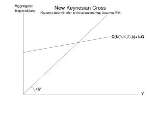
Equilibrium Aggregate Output (Income) • Equilibrium occurs when there is no tendency for change. In the macroeconomic goods market, equilibrium occurs when planned aggregate expenditure is equal to aggregate output.
Equilibrium AggregateOutput (Income) aggregate output /Yplanned aggregate expenditure /AE/C + Iequilibrium: Y = AE, or Y = C + I Disequilibria: Y > C + I aggregate output > planned aggregate expenditureinventory investment is greater than plannedactual investment is greater than planned investment C + I > Yplanned aggregate expenditure > aggregate outputinventory investment is smaller than plannedactual investment is less than planned investment
(1) (2) (3) Equilibrium AggregateOutput (Income) There is only one value of Y for which this statement is true. We can find it by rearranging terms: By substituting (2) and (3) into (1) we get:
The Saving/InvestmentApproach to Equilibrium If planned investment is exactly equal to saving, then planned aggregate expenditure is exactly equal to aggregate output, and there is equilibrium.
The S = I Approach to Equilibrium • Aggregate output will be equal to planned aggregate expenditure only when saving equals planned investment (S = I).
The Multiplier • The multiplier is the ratio of the change in the equilibrium level of output to a change in some autonomous variable. • An autonomous variable is a variable that is assumed not to depend on the state of the economy—that is, it does not change when the economy changes. • In this chapter, for example, we consider planned investment to be autonomous.
The Multiplier • The multiplier of autonomous investment describes the impact of an initial increase in planned investment on production, income, consumption spending, and equilibrium income. • The size of the multiplier depends on the slope of the planned aggregate expenditure line.
The Multiplier Equation • The marginal propensity to save may be expressed as: • Because DS must be equal to DI for equilibrium to be restored, we can substitute DI for DS and solve: therefore, , or
The Multiplier • After an increase in planned investment, equilibrium output is four times the amount of the increase in planned investment.
The Size of the Multiplierin the Real World • The size of the multiplier in the U.S. economy is about 1.4. For example, a sustained increase in autonomous spending of $10 billion into the U.S. economy can be expected to raise real GDP over time by $14 billion.
The Paradox of Thrift • When households become concerned about the future and decide to save more, the corresponding decrease in consumption leads to a drop in spending and income. • Households end up consuming less, but they have not saved any more.
Government Expenditures and Autonomous Net Taxes • We will assume that government expenditures (G) and net taxes (T) are autonomous • This assumption will keep our models from becoming overly complex • It will also allow us to easily analyze fiscal policy as both G and T change • It would be possible to consider taxes that vary with GDP (income taxes) $ G T Real income
Autonomous Net Exports (X - M) • If both exports (X) and imports (M) are autonomous, then net exports are autonomous $ X’’-M’’ X-M X’-M’ Real disposable income
Determinants of X-M • The following will cause a shift in the net export function. • The Exchange Rate • If the Dollar appreciates, then exports fall and imports rise, both causing net exports to fall, or shift down. • Foreign GDP (Income) • As foreign income rises, they import more goods from around the world including the US. So our exports will rise as we satisfy their demand for our goods.
Variable Imports • Imports may very well be related to income • This makes net exports decrease with income $ X-M Real disposable income
Planned Expenditures • What about the behavior (the “plans”) of our economic actors? • Consumption (C) is “planned” on the basis of disposable income • Investment (I) is “planned” based on the interest rate and business expectations (although it is autonomous with respect to GDP, or income) • G and (X-M) are simply autonomous • According to Keynes, aggregate planned expenditures (demand) determine output and income, even in the long run
The Income-Expenditure Model • A relationship between aggregate income and planned aggregate expenditures that determines, for a given price level, where income (and GDP) equals planned expenditures • The aggregate expenditure function is a relationship showing the amount of planned spending for each level of income • Equilibrium occurs in the model where planned aggregate expenditures equal income (GDP) • Unintended changes in inventories play a key role
Deriving Equilibrium Income and Output $ 45o C+I+G+(X-M) Equilibrium Real GDP Real GDP
The Simple Spending Multipliers $ C+I’+G+(X-M) 45o C+I+G+(X-M) I Simple spending multiplier = GDP/I = 1/(1-MPC) = 1/MPS Real GDP GDP
Keynes and the Great Depression • John Maynard Keynes argued that prices and wages are not sufficiently flexible to ensure the full employment of resources • Furthermore, Keynes argued that when resources (especially labor) are not fully employed (due to a lack of private investment expenditures), the government could provide offsetting expenditures as a means of stabilizing the economy • Thus, Keynesian economics places emphasis on planned expenditures and all its components
Appendix • Slides after this point will most likely not be covered in class. However they may contain useful definitions, or further elaborate on important concepts, particularly materials covered in the text book. • They may contain examples I’ve used in the past, or slides I just don’t want to delete as I may use them in the future.