Download
1 / 47
470 likes | 618 Vues
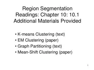
Region Segmentation Readings: Chapter 10: 10.1 Additional Materials Provided. K-means Clustering (text) EM Clustering (paper) Graph Partitioning (text) Mean-Shift Clustering (paper). Image Segmentation. Image segmentation is the operation of partitioning an

E N D
Region SegmentationReadings: Chapter 10: 10.1Additional Materials Provided K-means Clustering (text) EM Clustering (paper) Graph Partitioning (text) Mean-Shift Clustering (paper)
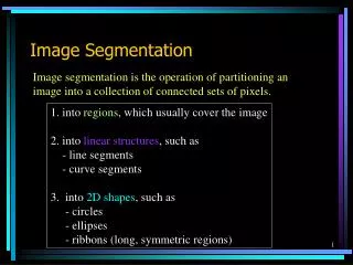
Image Segmentation Image segmentation is the operation of partitioning an image into a collection of connected sets of pixels. 1. into regions, which usually cover the image 2. into linear structures, such as - line segments - curve segments 3. into 2D shapes, such as - circles - ellipses - ribbons (long, symmetric regions)
Main Methods of Region Segmentation • 1. Region Growing • 2. Split and Merge • 3. Clustering
Clustering • There are K clusters C1,…, CK with means m1,…, mK. • The least-squares error is defined as • Out of all possible partitions into K clusters, • choose the one that minimizes D. K 2 D = || xi - mk || . k=1 xi Ck Why don’t we just do this? If we could, would we get meaningful objects?
K-Means Clustering Form K-means clusters from a set of n-dimensional vectors 1. Set ic (iteration count) to 1 2. Choose randomly a set of K means m1(1), …, mK(1). 3. For each vector xi compute D(xi , mk(ic)), k=1,…K and assign xi to the cluster Cj with nearest mean. 4. Increment ic by 1, update the means to get m1(ic),…,mK(ic). 5. Repeat steps 3 and 4 until Ck(ic) = Ck(ic+1) for all k.
K-means Variants • Different ways to initialize the means • Different stopping criteria • Dynamic methods for determining the right number of clusters (K) for a given image • The EM Algorithm: a probabilistic formulation of K-means
xi C(xi) K-Means • Boot Step: • Initialize K clusters: C1, …, CK Each cluster is represented by its mean mj • Iteration Step: • Estimate the cluster for each data point • Re-estimate the cluster parameters
K-Means Example Where do the red points belong?
K-means vs. EM K-means EM Cluster mean mean, variance, Representation and weight Cluster randomly select initialize K Initialization K means Gaussian distributions Expectation assign each point soft-assign each point to closest mean to each distribution Maximization compute means compute new params of current clusters of each distribution
Notation N( , ) is a 1D normal (Gaussian) distribution with mean and standard deviation (so the variance is 2.
N(, ) is a multivariate Gaussian distribution with mean and covariance matrix . What is a covariance matrix? R G B R R2 RG RB G GR G2 GB B BR BG B2 variance(X): X2 = (xi - )2 (1/N) cov(X,Y) = (xi - x)(yi - y) (1/N)
1. Suppose we have a set of clusters: C1, C2, ... , CK • over a set of data points X = {x1, x2, ... , xN}. • P(Cj) is the probability or weight of cluster Cj. • P(Cj | xi) is the probability of cluster Cj given point xi. • P(xi | Cj) is the probability of point xi belonging to • cluster Cj. • Suppose that a cluster Cj is represented by a • Gaussian distribution N(j,j). Then for any point xi:
For each cluster j EM: Expectation-Maximization • Boot Step: • Initialize K clusters: C1, …, CK • Iteration Step: • Estimate the cluster of each data point • Re-estimate the cluster parameters (j,j) and P(Cj)for each cluster j. Expectation Maximization
1-D EM with Gaussian Distributions • Each cluster Cj is represented by a Gaussian distribution N(j , j). • Initialization: For each cluster Cj initialize its mean j , variance j2, and weight j. N(2 , 2) 2 = P(C2) N(3 , 3) 3 = P(C3) N(1 , 1) 1 = P(C1)
Expectation • For each point xi and each cluster Cj compute P(Cj | xi). • P(Cj | xi) = P(xi | Cj) P(Cj ) / P(xi) • P(xi) = P(xi | Cj) P(Cj) • Where do we get P(xi | Cj) and P(Cj)? j
Use the pdf for a normal distribution: • Use j = P(Cj) from the current • parameters of cluster Cj.
Maximization • Having computed P(Cj | xi) for each point xi and each cluster Cj, use them to compute new mean, variance, and weight for each cluster. j2= j
Multi-Dimensional Expectation Stepfor Color Image Segmentation Input (Known) Input (Estimation) Output x1={r1, g1, b1} x2={r2, g2, b2} … xi={ri, gi, bi} … Cluster Parameters (1,1), p(C1) for C1 (2,2), p(C2) for C2 … (k,k), p(Ck) for Ck Classification Results p(C1|x1) p(Cj|x2) … p(Cj|xi) … +
Multi-dimensional Maximization Stepfor Color Image Segmentation Input (Known) Input (Estimation) Output x1={r1, g1, b1} x2={r2, g2, b2} … xi={ri, gi, bi} … Classification Results p(C1|x1) p(Cj|x2) … p(Cj|xi) … Cluster Parameters (1,1), p(C1) for C1 (2,2), p(C2) for C2 … (k,k), p(Ck) for Ck +
Full EM AlgorithmMulti-Dimensional • Boot Step: • Initialize K clusters: C1, …, CK • Iteration Step: • Expectation Step • Maximization Step (j,j) and P(Cj)for each cluster j.
Visualizing EM Clusters ellipses show one, two, and three standard deviations mean
EM Demo • Demo http://www.neurosci.aist.go.jp/~akaho/MixtureEM.html • Example http://www-2.cs.cmu.edu/~awm/tutorials/gmm13.pdf
EM Applications • Blobworld: Image segmentation using Expectation-Maximization and its application to image querying • Yi’s Generative/Discriminative Learning of object classes in color images
Jianbo Shi’s Graph-Partitioning • An image is represented by a graph whose nodes • are pixels or small groups of pixels. • The goal is to partition the vertices into disjoint sets so • that the similarity within each set is high and • across different sets is low.
Minimal Cuts • Let G = (V,E) be a graph. Each edge (u,v) has a weight w(u,v) • that represents the similarity between u and v. • Graph G can be broken into 2 disjoint graphs with node sets • A and B by removing edges that connect these sets. • Let cut(A,B) = w(u,v). • One way to segment G is to find the minimal cut. uA, vB
Cut(A,B) cut(A,B) = w(u,v) uA, vB B A w1 w2
Normalized Cut Minimal cut favors cutting off small node groups, so Shi proposed the normalized cut. cut(A, B) cut(A,B) Ncut(A,B) = ------------- + ------------- asso(A,V) asso(B,V) normalized cut asso(A,V) = w(u,t) uA, tV How much is A connected to the graph as a whole.
Example Normalized Cut B A 2 2 2 2 2 2 2 2 4 3 2 1 1 2 2 3 3 3 Ncut(A,B) = ------- + ------ 21 16
Shi turned graph cuts into aneigenvector/eigenvalue problem. • Set up a weighted graph G=(V,E) • V is the set of (N) pixels • E is a set of weighted edges (weight wij gives the similarity between nodes i and j) • Length N vector d: di is the sum of the weights from node i to all other nodes • N x N matrix D: D is a diagonal matrix with d on its diagonal • N x N symmetric matrix W: Wij = wij
Let x be a characteristic vector of a set A of nodes • xi = 1 if node i is in a set A • xi = -1 otherwise • Let y be a continuous approximation to x • Solve the system of equations (D – W) y = D y for the eigenvectors y and eigenvalues • Use the eigenvectorywith second smallest eigenvalue to bipartition the graph (y => x => A) • If further subdivision is merited, repeat recursively
How Shi used the procedure Shi defined the edge weights w(i,j) by w(i,j) = e * -||X(i)-X(j)||2 / X e if ||X(i)-X(j)||2 < r 0 otherwise -||F(i)-F(j)||2 / I where X(i) is the spatial location of node i F(i) is the feature vector for node I which can be intensity, color, texture, motion… The formula is set up so that w(i,j) is 0 for nodes that are too far apart.
Examples of Shi Clustering See Shi’s Web Page http://www.cis.upenn.edu/~jshi/
Problems with EM Problems with Graph Cuts • Need to know when to stop • Very Slooooow • Local minima • Need to know number of segments • Need to choose generative model
Mean-Shift Clustering • Simple, like K-means • But you don’t have to select K • Statistical method • Guaranteed to converge to a fixed number of clusters.
Finding Modes in a Histogram • How Many Modes Are There? • Easy to see, hard to compute
Mean Shift [Comaniciu & Meer] • Iterative Mode Search • Initialize random seed, and window W • Calculate center of gravity (the “mean”) of W: • Translate the search window to the mean • Repeat Step 2 until convergence
Numeric ExampleMust Use Normalized Histogram! window W centered at 12 mean shift x H(x) 5 4 3 2 1 N(x) 5/15 4/15 3/15 2/15 1/15 10 11 12 13 14 • x N(x) = 10(5/15)+11(4/15)+12(3/15)+13(2/15)+14(1/15) • = 11.33
Mean Shift Approach • Initialize a window around each point • See where it shifts—this determines which segment it’s in • Multiple points will shift to the same segment
Segmentation Algorithm • First run the mean shift procedure for each data point x and store its convergence point z. • Link together all the z’s that are closer than .5 from each other to form clusters • Assign each point to its cluster • Eliminate small regions
Mean-shift for image segmentation • Useful to take into account spatial information • instead of (R, G, B), run in (R, G, B, x, y) space
References • Shi and Malik, “Normalized Cuts and Image Segmentation,” Proc. CVPR 1997. • Carson, Belongie, Greenspan and Malik, “Blobworld: Image Segmentation Using Expectation-Maximization and its Application to Image Querying,” IEEE PAMI, Vol 24, No. 8, Aug. 2002. • Comaniciu and Meer, “Mean shift analysis and applications,” Proc. ICCV 1999.