Small Josephson Junctions in Resonant Cavities
340 likes | 587 Vues
H2.005. Small Josephson Junctions in Resonant Cavities. David G. Stroud , Ohio State Univ. Collaborators: W. A. Al-Saidi, Ivan Tornes, E. Almaas Work supported by NSF DMR01-04987.

Small Josephson Junctions in Resonant Cavities
E N D
Presentation Transcript
H2.005 SmallJosephsonJunctionsinResonantCavities David G. Stroud, Ohio State Univ. Collaborators: W. A. Al-Saidi, Ivan Tornes, E. Almaas Work supported by NSF DMR01-04987 Motivation: to develop models for controllable two-level superconducting systems for possible use in quantum computation
What is a Josephson Junction? • A Josephson junction is a weak link between two strong superconductors • Small junction: typically region between superconductors is insulating (i); junction underdamped I Current I I i s s
Hamiltonianofa smallJosephsonjunction • Let be the phase difference across a junction • Let n be the difference in the number of Cooper pairs on the two superconducting islands • Then the Hamiltonian of the junction is • where U= /C is the charging energy and J is the Josephson coupling energy. (C=capacitance)
Commutationrelations Schrodingerequationis where Wave function which solves this equation is that of a particle of massmovingin acosinepotential
Voltage-biasedJosephsonjunction • If junction is voltage-biased,the kinetic energy term in the Hamiltonian becomes IfJosephsonenergyvanishes, energy eigenvalues are just With n = 0, 1, 2,…..
Schematic of voltage-biasedjunction Cg=gate capacitance; Vg=gate voltage Junction Hamiltonian is
Schrodingerequationforvoltage-biasedsmalljunction Solvetoobtaineigenvaluesandwavefunctionsasfunctionsof Experiment: junction can be placed in macroscopic superposition of twodistincteigenstates[e. g. Bouchiatetal, Phys.Scr.T76,165(1998); Nakamuraetal, PRL79, 2328(1997);Nature398, 786 (1999); Zorinetal, cond-mat/0105211]
Single-Mode Resonant cavity Cavityfields E,B HamiltonianofResonant Cavity Mode is Hereisthecavityfrequency,a and a+ arephotonannihilation/creationoperators.Energiesare(m+1/2)
Cavity-junction interaction In presence of a vector potential, phase difference in expression for Josephson energy is replaced by a gauge-invariant phase difference: Here g represents the junction-cavity coupling strength, and is related to the cavity vector potential in the junction
Strengthofjunction-cavitycoupling Note: lineintegraltakenacrossjunction Normalized cavity electric field = Cavity frequency Flux quantum (= hc/2e) Thus, maximum coupling occurs when E-field is concentrated in as small a volume as possible
Schematic illustration of geometry for a voltage-biasedJosephsonjunctionina microcavity I Supercon Supercon S S I I I II S Microcavity Josephsonjunctionistwosuperconductors (SandS) separatedbyinsulatingregion
Solutionofcombinedjunction-cavityproblem • Compute Hamiltonian matrix in product basis |km> of junction and cavity states (k=0,1,2,…= junction states; m=0,1,2…= cavity states) • Diagonalize to obtain eigenvalues and eigenfunctions as functions of g, offset voltage, cavity frequency, etc. • At certain values of offset voltage, states of cavity and junction are highlyentangled – i. e., cannot be written as products of cavity and junction states.
Energy level diagram for junction-cavity system Lowest eigenvalues E/U of the junction-cavity system, plotted as a function of for the following parameters: /U=0.3, J/U=0.7, and several values of g as indicated. Twoarrowsindicatepairsofdegeneratestates [Al-Saidi and Stroud, PRB65, 014512 (2002)].
Time-dependentbehaviorofJosephson-cavitysystem, =0.26 [Obtainedbysolvingtime-dep’tSchrodingerequationstartingfrom|k=0,m=1>] Left: energy in junction (solid line) and in cavity (dashed line) versus time. Right: probability that junction is in first excited state (full line) and that the cavity is in m=1 (one-photon) state (dashed line). Calculation includes ALL the quantum states of junction and cavity. Cavity oscillates between m =0 and m = 1.
Josephson-cavity system, = 0.06 Same as previous picture, except that offset voltage is tuned so that junction oscillates between ground and first excited state, and cavity oscillates between m=0 and m=2 states.
Two-level approximation • Calculate Rabi frequency including only the two nearly degenerate states. • For = 0.26, these are |k=0;m=1> and |k=1;m=0>. For = 0.06, they are |k=0,m=2> and |k=2;m=0>. • For the first case, 2-state approx. gives a Rabi frequency within 1% of exact calculation. For second case, it gives a Rabi frequency within 20% of exact calc.
”Collapseandrevival” [coined by J. H. Eberley et al, PRL 44, p. 1323 (1980)] Full curve: Time-dependentprobability that junction in first excited state, given resonator initially in a “coherent state” (coherent superposition of different number states) and junction in ground state. Dashedcurve: junction treated in two-level approximation, but all photon states included. [Al-Saidi and Stroud, Phys. Rev. B65, 014512 (2002).]
[E. T. Jaynes and F. W. Cummings, Proc. IEEE 51, 89 (1963)] Jaynes-Cummings Model Hamiltonian for a two-statesystem coupled to a singlemode of a quantized electromagnetic field (or any single mode oscillator): Energy splitting of two lowest levels are components of spin-1/2 operators Our numerical results using fullHamiltonian for junction-cavity system very close to Jaynes-Cummings results including only twolowestjunctionlevels.
Remarksaboutsinglejunctioncoupledtosingle-modecavity • Quantum behavior closely resembles that of two-statesystem coupled to cavitymode, at certain values of offset voltage • Junction does NOT have to be a charging-energy dominated*; charging and Josephson energy can be comparable *Regime studied by Shnirman et al, PRL79, 2371 (1997) and by Buisson and Hekking, cond-mat/0008275.
SeveralJunctionsin aResonantCavity • Is it possible to couple several Josephson junctions to the SAME resonant cavity? • Yes! The mathematical model is very similar to one used to treat severalidenticaltwo-levelatoms placed in the sameresonantcavity: the Dicke model [R. H. Dicke, 1954] • The models would be identical if the junctions were truly two-level systems, but this is true only approximately
ModelHamiltonianforSeveral-JunctionProblem =cavityHamiltonian =Hamiltonianforjthjunction =Hamiltonianforjunction-cavityinteraction
Dickemodel • TheHamiltonianfortheDickemodelis Here a and are the annihilation and creation operators for the photon mode, S’s are components of the spin-1/2 operators, and = strength of coupling between the two-level system and the cavity mode. Junction-cavitysystem differs from the Dicke model because junctions are non-identical and non2-level systems.
Rabi oscillations in a system of several junctions in a cavity This Figure plots the time-dependent “inversion” S(t) (sum of probabilities that each junction is in its excited state) for systems of 2 and 4 junctions in a resonant cavity, given that initially exactly one junction is excited. Rabi frequency is approximately proportional to square root of number of junctions. [CalculatedusingfullHamiltonian] (Al-Saidi and Stroud, Phys. Rev. B65, 224512 (2002).)
S(t) for coherent initial state, one and two junctions Time-dependent “inversion” S(t) (=sum of probabilities that each junction is in its excited state) for (a) N = 1 and (b) N = 2 junctions, given that resonator is initially in a “coherent” state (eigenstate of annihilation operator), and junctions in their ground state. Solidlines: fullnumericalsolution; dashedlines, two-levelapproximation. The two junctions are assumed identical.
Remarksaboutsystemofseveraljunctionsin acavity • Two-level (Dicke) approximation works quite well. • Influence of higher levels can be incorporated into an effectivedipole-dipoleinteraction between the “qubits”: • If junctionsarenon-identical, there are still Rabi oscillations (frequency proportional to square root of junction number) if junctions slightly different. For larger differences, each junction couples independently to the cavity. • In “classicallimit” (many photons), dynamical equations predict “self-inducedresonantsteps” in the IV characteristics (Almaas and Stroud, 2002) in agreement with expt (Barbara et al, PRL, 1999).
LongJosephson “ring” withcrossedstaticandcavitymagneticfields H VortexinringbehaveslikeCooperpairinsmalljunction I I I v Vortex in ring is like a magnetic moment interacting with magnetic fields Cavitymagneticfield H’
Qubitfromvortexcoupledtocavitymagneticfield • Magneticmomentofvortexcouplestoapplied static magnetic field +magnetic fieldof cavity. • When current is applied across the ring, vortex is driven around the ring. Applied static magnetic field produces cosine potential.* • With magnetic field of cavity mode, quantum Hamiltonian of system is formally identical (for small vortex velocities) to that of small junction • Hence, should be able to make qubit analogous to that produced by small junction coupled to a cavity mode (but via magnetic, notelectric, fields. Quantum mechanics in case of static field already seen in experiments, and calculated by Wallraff et al (Nature vol.425, p. 6954 2003).
Hamiltonian for vortex-cavity system • Hamiltonian is (for slow vortex) H= FormofHamiltonianisidenticaltothatofsmalljunctioncoupledtoelectricfieldofcavity
Summary • Have computed quantum states of states of Josephsonjunctionscoupledtosingle-modecavities. • Junctions may behave like two-levelsystems which can be stronglyentangled with cavity states. • Severaljunctionsin acavity, can behave like groups of controllable two-level systems which can be entangled via the cavity. • Work in progress: (i) Othergeometries for two level systems; (ii) couplingviamagneticfields of cavity modes; (iii) calculation of dissipation.