Download
1 / 24
240 likes | 270 Vues
Explore the impact of frequency domain phenomena on time domain digital signals. Learn about decomposing digital signals, frequency components, and estimating frequency content. Study how to apply frequency-dependent effects and examine methods of generating square waves.

E N D
Interconnect II – Class 22 Prerequisite Reading - Chapter 4
Effects of Frequency Domain Phenomena on Time Domain Digital Signals • Key Topics: • Frequency Content of Digital Waveforms • Frequency Envelope • Incorporating frequency domain effects into time domain signals Interconnect II
Decomposing a Digital Signal into Frequency Components • Digital signals are composed of an infinite number of sinusoidal functions – the Fourier series • The Fourier series is shown in its progression to approximate a square wave: 1 + 2 + 3 1 + 2 1 1 0 - 2 3 1 + 2 + 3 + 4 + 5 1 + 2 + 3 + 4 Square wave: Y = 0 for - < x < 0 and Y=1 for 0 < x < Y = 1/2 + 2/pi( sinx + sin3x/3 + sin5x/5 + sin7x/7 … + sin(2m+1)x/(2m+1) + …) 1 2 3 4 5 May do with sum of cosines too. Interconnect II
Tr 20dB/decade Pw T 40dB/decade Harmonic Number …... 1 5 9 3 7 Frequency Content of Digital Signals • The amplitude of the the sinusoid components are used to construct the “frequency envelope” – Output of FT Interconnect II
Estimating the Frequency Content • Where does that famous equation come from? • It can be derived from the response of a step function into a filter with time constant tau • Setting V=0.1Vinput and V=0.9Vinput allows the calculation of the 10-90% risetime in terms of the time constant • The frequency response of a 1 pole network is • Substituting into the step response yields Interconnect II
Estimating the Frequency Content Edge time factor • This equation says: • The frequency response of the network with time constant tau will degrade a step function to a risetime of t10-90% • The frequency response of the network determines the resulting rise time ( or transition time) • The majority of the spectral energy will be contained below F3dB • This is a good “back of the envelope” way to estimate the frequency response of a digital signal. • Simple time constant estimate can take the form L/R, L/Z0, R*C or Z0*C. Interconnect II
Examining Frequency Content of Digital Signals • The frequency dependent effects described earlier in this class can be applied to each sinusoidal function in the series • Digital signal decomposed into its sinusoidal components • Frequency domain transfer functions applied to each sinusoidal component • Modified sinusoidal functions are then re-combined to construct the altered time digital signal • There are several ways to determine this response • Fourier series (just described) • Fast Fourier transform (FFT) • Widely available in tools such as excel, Mathematica, MathCad… Interconnect II
3 Method of Generating a Square Wave • Ramp pulses • Use Heavy Side function • Used for first pass simulations • Power Exponential Pulses • Realistic edge that can match silicon performance • Used for behavioral simulation that match silicon performance. • Sum of Cosines • Text book identity. • Used to get a quick feel for impact of frequency dependant phenomena on a wave. Interconnect II
Ramp Square Wave Interconnect II
Power Exponential Square Wave Interconnect II
Sum Cosine Square Wave Interconnect II
Applying Frequency Dependent Effects to Digital Functions Input signal into lossy t-line Spectral content of waveform FT FFT Volts Frequency Time Time domain waveform with frequency dependent losses Multiply Loss characteristics if t-line With AC losses No AC losses Inverse FFT Volts Attenuation (V2/V1) Time Frequency AC losses will degrade BOTH the amplitude and the edge rate Interconnect II
Use MathCad to create a pulse wave with Sum of sine waves Sum of ramps Sum of realistic edge waveforms Exponential powers Use MathCad to determine edge time factor for exponential and Gaussian wave, 10% - 90% 20% - 80% Assignment Interconnect II
Remember this equation from a few slides ago? • This equation says: • If a step response is driven into a filter with tine constant tau, the output edge rate is t10-90% • However, realistic edge rates are not step functions • RSS the input edge rate with the filter response Input edge tr = 300ps Example: tout=Output edge Zo=50 C=5pF Edge Rate Degradation due to filtering Interconnect II
Additional Effects • Key Topics: • Serpentine traces • Bends • ISI • Topology Interconnect II
Lp S Effects of a Serpentine Trace • Serpentine traces will exhibit 2 modes of propagation • Typical “straight line” mode • Coupled mode via the parallel sections • Causes the signal to “speed up” because a portion of the signal will propagate perpendicular to the serpentine • ”Speed up” is dependent on the spacing and the length Interconnect II
Modeling Serpentines • Assignment – Find a the uncoupled trace length that matches the delay of the serpentine route below • Use Maxwell Spice/2D modeling of serpentine vs. equal length wave. Trace route on PWB • 1 oz copper • 5 mil space • 5mil width • 5 mil distance to ground plane • Symmetric stripline • Use 50 ohm V source w/ 1ns rise time (do for ramp and Gaussian) 1” 2 port Tline model 5 mil 2 port Tline Model 10 port Transmission Line SpiceModel Couple length=2 inches Interconnect II
Rules of Thumb for Serpentine Trace • The following suggestions will help minimize the effect of serpentine traces • Make the minimum spacing between parallel section (s) at least 3-4H, this will minimize the coupling between parallel sections • Minimize the length of the parallel sections (Lp) as much as possible • Embedded microstrips and striplines exhibits less serpentine effects than normal m9ictrostirpsd Interconnect II
Effects of bends • Virtually every PCB design will exhibit bends • The excess area caused by a 90o bend will increase the self capacitance seen at the bend • Empirically inspired model of a 90o bend is simply 1 square of excess capacitance Capacitance of 1 extra square • Measurements have shown increased delays due to the current components “hugging” the corner increasing the mean length • 2 rights do not necessarily equal a left and a right, especially for wide traces • 45o bends, round and chamfered bends exhibit reduced effects Interconnect II
Inter Symbol Interference • Inter symbol interference (ISI) is reflection noise that effects both amplitude and timing • The nature of this interference is cause by a signal not settling to a steady stated value before the next transition occurs. • Can have an effect similar to crosstalk but has completely different physics Volts Ideal waveform beginning transition from low to high with no reflections or losses Timing difference Waveform beginning transition from low to high with unsettled noise cased by reflections. Receiver switching threshold Time Different starting point due to ISI Interconnect II
400 MHz switching 200 MHz switching Ideal 400 MHz waveform Inter Symbol Interference • ISI can dramatically affect the signal quality • Depending on the switching rate/pattern, significant differences in waveform shape can be realized – one or two patterns won’t produce worst case • If the designer does not account for this effect, switching patterns that are unaccounted for result in latent product defects. Interconnect II
What about the case where there is more than one receiver, or more than one driver (e.g., a Multi-processor FSB) Zo2 Receiver 1 L1 Rs=Zo L2 (L1=L2) Zo1 L3 0-2V Vs Zo3 Receiver 2 • There will be an impedance discontinuity at the junction • The equivalent input impedance looking into the junction will be the parallel combination of Zo2 and Zo1 • This model can be simplified and solved with lattice diagrams • Valid when L1=L2 Rs=Zo L2 L1 Zo1 Z=Zo2||Zo3 Vs 0-2V Topology – the Key to a sound design Interconnect II
The reflections from the receiver discontinuities will not arrive at the same time; the 2 segment simplification is not applicable • This topology will ring with a frequency dependant in L2 and L3 • This topology can be solved with a multi-segment lattice diagram Topology – the Key to a sound design • Now, consider the case where L2 and L3 are NOT Equal Receiver 1 Zo2 Rs=Zo L2 L3 Zo1 0-2V Vs Zo3 Receiver 2 Interconnect II
R1 Zo Rs=Zo J In Zo 0-2V Vs Zo R 2 Topology – the Key to a sound design A A’ B B’ C In J R1 R2 Interconnect II