Polynomials and the Fast Fourier Transform (FFT)

1. Polynomials and the Fast Fourier Transform (FFT)

2. Polynomials and the Fast Fourier Transform (FFT) [Cormen pp 898-925] • The straightforward method takes • Θ(n) time for adding two polynomials of degree n, and • Θ(n2 ) time for multiplying them. • We will show how the fast Fourier transform (FFT) can reduce the time to Θ(n log n) for multiplying polynomials. • Applications of FFT’s are compression techniques used to encode digital video and audio information, including MP3 files, as well as in signal processing. MP3 (formally MPEG-1 Audio Layer III or MPEG-2 Audio Layer III)is an audio coding format for digital audio. 

3. Polynomials A polynomial in the variable over an algebraic field F represents a function A() as a formal sum: A() = That is, A() = . We call the values the coefficients of the polynomial. The coefficients are drawn from a field F, typically the set Ƈ of complex numbers. r

4. Let A(x) = xn-1 + xn-2 + …+ A polynomial A() has a degree n-1 if its highest nonzero coefficient is ; we write that degree (A) = n-1. Any integer n strictly greater than the degree of a polynomial is a degree-bound of that polynomial. The degree of a polynomial of degree-bound n may be any integer between 0 and n – 1, inclusive. [think? n > n-1, n-2, …, 2, 1, 0! n terms.]

5. Operations on Polynomials • Polynomial addition: • Polynomial multiplication:

6. Polynomial addition: If A(x) and B(x) are polynomials of degree-bound n, their sum is a polynomial C(x), also of degree-bound n, such that C(x) = A(x) + B(x) for all x in the underlying field. The brute-force algorithm for adding two polynomials is: if A(x) = and B(x) = then C(x) = where cj = aj + bj for j = 0, 1, 2, …, n – 1.

7. Let a(x) = xn-1 + xn-2 + …+ Let b(x) = xn-1 + xn-2 + …+ Adding polynomials representing by the coefficient vectors and takes Θ(n) time to produce the vector , where for j = 0, 1, 2, …, n-1. To compute C(x) = where cj = aj + bj for j = 0, 1, 2, …, n – 1.

8. Example 2.18: A(x) = 6x3 + 7x2 - 10x + 9 i.e., (9, -10, 7, 6) B(x) = -2x3 + 4x - 5 + i.e., (-5, 4, 0, -2) C(x) = 4x3 + 7x2 - 6x + 4. i.e., (9+(-5), (-10)+4, 7+0, 6+(-2)) encoded using 2’ complement as strings of 0 and 1 with 1 in the sign bit

9. Let a(x) = xn-1 + xn-2 + …+ Polynomial multiplication: If A(x) and B(x) are polynomials of degree-bound n, their product is a polynomial C(x), also of degree-bound 2n - 1, such that C(x) = A(x)B(x) for all x in the underlying field. Multiply each term in A(x) by each term in B(x), and then combine terms with equal powers. The brute-force algorithm for multiplying two polynomials is: if A(x) = and B(x) = C(x) = ………………….. (2.13) where cj = ………………….. (2.14) Let b(x) = xn-1 + xn-2 + …+ A and B are degree-bound n. Their product is of degree-bound 2n-1. *

10. a = () of degree bound n for of degree n-1 x b = () of degree bound n for of degree n-1 ____________________________________________________________ of degree bound 2n-1 for of degree 2n-2 and the term with highest degree is = x . The total number of term of the product is 2n-1 and therefore is degree bound 2n-1.

11. C(x) = where cj = c0 = c1 = + c2 = + + c2 = + + … • A and B are degree-bound n. • i.e., each of A and B has n=4 terms. • They are of degree n-1 which is 3. • Their product is of degree-bound 2n-1. • e.g.,The product of A*B has 7 terms. • It is of degree 2n-2 (i.e., 6). • Example 2.19 6x3 + 7x2 - 10x + 9 • - 2x3+ 0x2 + 4x - 5 - 30x3 - 35x2 + 50x - 45 - 24x4 - 28x3- 40x2 - 36x • + 0x5+ 0x4 + 0x3 + 0x2 - 12x6 - 14x5 + 20x4 - 18x3 . - 12x6 - 14x5 + 44x4 - 20x3 - 75x2 + 86x - 45

12. X * i.e., (na – 1) + (nb – 1) = na + nb – 2 For C = A * B, that degree(C) = degree(A) + degree(B), implying that if A is a polynomial of degree-bound na (i.e., A has na terms) and B is a polynomial of degree-bound nb (i.e., B has nb terms) , thenC is a polynomial of degree-bound na + nb – 1. That means C has na + nb – 1 terms of degree na + nb – 2. Since a polynomial of degree-bound k is also a polynomial of degree-bound k + 1, we will normally say that the product polynomial C is a polynomial of degree-bound na + nb.

13. n = 4 Example 2.20 a3 x3 + a2 x2 + a1 x1 + a0 x0 * b3 x3 + b2 x2 + b1 x1 + b0 x0 a3b0 x3 + a2b0 x2 + a1b0 x1 + a0b0 x0 a3b1 x4 + a2b1 x3 + a1b1 x2 + a0b1 x1 a3b2 x5 + a2b2 x4 + a1b2 x3 + a0b2 x2 a3b3 x6 + a2b3 x5 + a1b3 x4 + a0b3 x3 a3b3 x6 + (a3b2 + a2b3)x5 + (a3b1 + a2b2 + a1b3 ) x4 + (a3b0 + a2b1 + a1b2+ a0b3 )x3 + (a2b0+ a1b1+ a0b2) x2 + (a1b0 + a0b1) x1 + a0b0 x0 n = 4 16 = 42multiplications (in general multiplying two polynomials, each of degree-bounded n, requires n2) plus 15 additions

14. If A(x) = and B(x) = then, a way to express the product C(x) = A(x) * B(x) is C(x) = ……………………………... (2.13) where cj = ………….………………….. (2.14)

15. For this case, n – 1 = 3. That is, n = 4. C(x) = = c0 x0 + c1 x1 + c2 x2 + c3 x3 + c4 x4 + c5 x5 + c6 x6 where cj = Consider a3 x3 + a2 x2 + a1 x1 + a0 x0 * b3 x3 + b2 x2 + b1 x1 + b0 x0 That is, For j = 0, then c0 = = a0b0. (9 * (-5)) For j = 1, then c1 = = a1b0 + a0b1. (-10 * -5 + 9 * 4) For j = 2, then c2 = = a2b0+ a1b1+ a0b2. (7 * -5 + -10 * 4 + 7 * 0) For j = 3, then c3 = = a3b0 + a2b1 + a1b2+ a0b3. For j = 4, then c4 = = a4b0 + a3b1 + a2b2 + a1b3 + a0b4. For j = 5, then c5 = = a5b0+ a4b1+ a3b2 + a2b3 + a1b4 + a0b5. For j = 6, then c6 = = a6b0+ a5b1+ a4b2+ a3b3 + a2b4 +a1b5 + a0b6. (6 * -2) Multiplying polynomials – equations (2.13) and (2.14) – take Θ(n2) time when we represent polynomials in coefficient form. That is, if n = 4, then n2 = 42 = 16 multiplies.

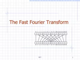
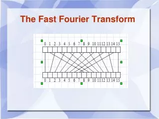
16. The straightforward methods for multiplying polynomials – equations (2.13) and (2.14) : • take Θ(n2) time when we represent polynomials in coefficient form,but • only Θ(n) time when we represent them in point-value form. • Converting polynomials between their coefficient representation and point-value representation, each requires Θ(n log n) time. • That is, by combining them, we can multiply two degree-bound n polynomials (in point-value forms) taking Θ(n log n) time. That is, Θ(n log n) + Θ(n) + Θ(n log n).

17. Comment: for x3, If n-1=3, then n=4 terms for x6, if 2n-1=6, then 2n=7 terms Ordinary Multiplication Time Θ(n2) a0 , a1, …, an-1 b0 , b1, …, bn-1 Coefficient representation c0 , c1, …, c2n-1 convolution Evaluation Interpolation Time Θ(n2), Time Θ(n2) using Horner Rule using Lagrange’s formula • … • … Pointwise multiplication Point-value multiplication Time Θ(n)

18. a = () + b = () c = (), where cj = aj + bj Coefficient representation A coefficient representation of a polynomial A(x) = of degree-bound n is a vector of coefficients a = (). In matrix equations, we shall generally treat vectors as column vectors. Adding two polynomials represented by the coefficient vectors a = () and b = () takes Θ(n) time: we simply produce the coefficient vector c = (), where cj = aj + bj for j = 0, 1, 2, …, n – 1.

19. Coefficient representation • Multiplying polynomials A(x) and B(x) in coefficient form • a = () and • b = () , • the resulting coefficient vector , given by equation • cj = (2.14) • called the convolutionof the input vectors a and b, denoted c = a b. • … • This takes Θ(n2) time for multiplying polynomials representing by the coefficient vectors and to produce the vector , where , k = 0, 1, 2, … j, for each j = 0, 1, 2, …, 2n-2.

20. Point-value representation A point-value representation of a polynomial A(x) of degree-bound n is a set of n point-value pairs {(x0 , y0), (x1 , y1), …, (xn - 1 , yn - 1)} such that all of the xk are distinct and yk = A(xk) ………………………..(2.15) for k = 0, 1, 2, …, n – 1. A polynomial has many different point-value representations, since we can use any set of n distinct points x0, x1, …, xn - 1 as a basis for the representation. y = A(x) = a3 x3 + a2 x2 + a1 x1 + a0 x0 yk= A(xk) = a3xk3 + a2xk2 + a1xk1 + a0xk0

21. Converting between Coefficient form and Point-value Representation Evaluating polynomial For computing a point-value representation for a polynomial given in coefficient form, arbitrarily select n distinct point x0 , x1 , …, xn - 1 and then evaluate A(xk) for k = 0, 1, 2, …, n – 1. The operation of evaluating the polynomial A(x) at a given point x0consists of computing the value of A(x0). We can evaluate a polynomial, saysA(x0),in Θ(n) time using Horner’s rule: A(x0) = ) … )). instead of a0+ a1 + a2 + … + an-1. yk = a3xk3 + a2xk2 + a1xk1 + a0xk0 yields yk = (((a3 ) xk+ a2 ) xk+ a1) xk+ a0

22. - each of these requires n multiply to get any of them. • … • - We have 2n terms for each of A and B. • These require 2(n*2n) ‘multiply’. With Horner’s method, evaluating a polynomial at n pointstake time Θ(n2) of multiplications. We shall see later that if we choose the points xk cleverly, we can accelerate this computation to run in time Θ(n log n). ….. [So far, converting coeficient form to point-value form]

23. Comment: for x3, If n-1=3, then n=4 terms for x6, if 2n-1=6, then 2n=7 terms Ordinary Multiplication Time Θ(n2) a0 , a1, …, an-1 b0 , b1, …, bn-1 Coefficient representation c0 , c1, …, c2n-1 Evaluation Interpolation Time Θ(n2), Time Θ(n2) using Horner Rule using Lagrange’s formula • … • … Pointwise multiplication Point-value multiplication Time Θ(n) To compute A*B

24. Example 2.21:Let consider the previous example again: Let A(x) be 6x3 + 7x2 - 10x + 9, and B(x) be - 2x3 + 4x - 5. Then the coefficient of A, the vector a = () is (9, -10, 7, 6) and the coefficient of B, the vector b = () is (-5, 4, 0, -2). The coefficient of C(x) = A(x) + B(x), the vector of c = () is (4, -6, 7, 4). Point-value representation of the polynomial A(x) of degree-bound 4 is a set of 4 point-value pairs: {(0, 9), (1, 12), (2, 65), (3, 204)} and B(X) of degree-bound 4 is {(0, -5), (1, -3), (2, -13), (3, -47)}, using Horner’s rule: A(x0) = ))) to compute. The point-value representation of C(x) = A(x) + B(x) = {(0, 4), (1, 9), (2, 52), (3, 157)} n-1 multiplications needed for degree-bound n. Since n of A, it requires n(n-1)) multiplications Instead of n() ) multiplications. Evaluation

25. Let A(x) be 6x3 + 7x2 - 10x + 9, and B(x) be - 2x3 + 4x - 5. Adding A(x) and B(x), we have C(x) = A(x) + B(x) = 4x3 + 7x2 - 6x + 5. Using Horner’s rule, their point-value representations can be computed by: A(x0) = ))), and B(x0) = ))). Since the polynomial A(x) of degree-bound 4, a set of 4 point-value pairs is needed for summation of A(x) and B(x): Pick arbitrarily x0 = {0, 1, 2, 3}. Then A(0) = 9, A(1) = 12, A(2) = 65, A(3) = 204, and B(0) = -5, B(1) = -3, B(2) = -13, B(3) = -47. Evaluation Point-value representations of A(x) is {(0, 9), (1, 12), (2, 65), (3, 204)} and of B(X) of degree-bound 4 is {(0, -5), (1, -3), (2, -13), (3, -47)}, and of C(x) is {(0, 4), (1, 9), (2, 52), (3, 157)} Point-value representations

26. Ordinary Multiplication Time Θ(n2) a0 , a1, …, an-1 b0 , b1, …, bn-1 Coefficient representation c0 , c1, …, c2n-1 • (4, -6, 7, 4) (9, -10, 7, 6) (-5, 4, 0, -2). addition EvaluationInterpolation Time Θ(n2), Time Θ(n2) using Horner Rule using Lagrange’s formula • … • … Pointwise multiplication Point-value multiplication Time Θ(n) (0, 9), (0, -5) (1, 12), (1, -3) (2, 65), (2, -13) (3, 207), (3, -47) (0, 4) (0, 9) (0, 52) (0, 157) To compute A*B

27. Interpolating polynomial - the inverse of evaluation (interpolation) The inverse of evaluation – determining the coefficient form of a polynomial from a point-value representation – is interpolation. Theorem 2.4 (Uniqueness of an interpolating polynomial) For any set {(x0 , y0), (x1 , y1), …, (xn - 1 , yn - 1)} of n point-value pairs such that all the xk values are distinct, there is a unique polynomial A(x) of degree-bound n such that yk = A(xk) for k = 0, 1, 2, …, n – 1. This Theorem shows that interpolation is well-defined when the desired interpolating polynomial must have a degree-bound equal to the given number of point-value pairs.

28. Evaluation: Another way to compute point-value representation of a polynomial Proof: The proof relies on the existence of the inverse of a certain matrix. Equation (2.15) yk = A(xk) is equivalent to the matrix equation (computing yk = A(xk), k = 0,1, …, n-1). 1 … 1 … 1 … , which yields 1 … = (2.16) a0+ a1 + a2 + … + an-1y0 a0+ a1 + a2 + … + an-1y1 a0+ a1 + a2 + … + an-1 = yk a0+ a1 + a2 + … + an-1yn-1 S yk = an-1a3xk3 + a2xk2 + a1xk1 + a0xk0 yields yk = (((…(an-1 ) xk+ … +a3) xk+ a2 ) xk+ a1) xk+

29. Example 2.22: Converting representation from point value pairs form to coefficient form: Consider A(x) = 6x3 + 7x2 - 10x + 9 and B(x) = - 2x3 + 4x - 5 . The coefficient form for the polynomial A(x) of degree-bound 4 is (9, -10, 7, 6). Use Horner’s rule A(x) = 9 + x(-10 + x(7 + x(6))) to compute its value-point form representation. Let x0 = {0, 1, 2, 3}. A(0) = 9. A(1) = 9 + 1(-10 + 1(7 + 1(6))) = 12 . A(2) = 9 + 2(-10 + 2(7 + 2(6))) = 65. A(3) = 9 + 3(-10 + 3(7 + 3(6))) = 204  We obtain its value-point form representation (0, 9), (1, 12), (2, 65), (3, 204). This above evaluating A(xk), k = 0, 1, 2, 3 can be done:

30. 1 0 0 0 9 9 • 1 1 1 -10 12 • 1 2 4 8 7 65 • 1 3 9 27 6 204 S = convolution/evaluation : Another way to compute point-value representations from coefficient vector for polynomial A(x) For A(x) = 6x3 + 7x2 - 10x + 9, the coefficient form for the polynomial A(x) of degree-bound 4 is (9, -10, 7, 6). Let x0 = {0, 1, 2, 3}. its value-point form representation (0, 9), (1, 12), (2, 65), (3, 204) can be obtained.

31. Given the point-value representation, Interpolating A(x) can be done: • 0 0 0 • 1 1 1 1 • 1 2 4 8 • 1 3 9 27 • Since det(V(x0 , x1 , …, xn - 1) ) • = • = (x1 – x0) (x2 – x0) (x3 – x0) (x2 – x1) (x3 – x1) (x3 – x2) • = (1 - 0)(2 - 0)(3 - 0)(2 - 1)(3 - 1)(3 - 2) = 1*2*3*1*2*1=12 • ≠ 0, it is nonsingular, • a = V(x0 , x1 , …, xn - 1)-1 * y. ……2.22 S V(0, 1, 2, 3) = As j goes from 0 to 2, k is from 1 to 3.

32. That is, a0 1 0 0 0 -1 9 9 a1 1 1 1 1 12 -10 a2 1 2 4 8 65 7 a3 1 3 9 27 204 6 S = = Interpolation: Another way to compute coefficient vector from point-value representations for polynomial A(x). This takesΘ(n3).

33. The proof of Theorem 2.4 describes an algorithm for interpolation based on solving the set y = V(x0 , x1 , …, xn - 1) * a (2.16) of linear equations. Using the LU decomposition algorithms, we can solve these equations in time Θ(n3).

34. Fast n-point interpolation algorithm – from point-value back to coefficients • A fast algorithm for n-point interpolation is based on Lagrange’s formula: • A(x) = …………… (2.17) • It can verify that • the right-hand side of equation (2.17) is a polynomial of degree-bound n that satisfies A(xk) = yk for all k. • compute the coefficients of A using Lagrange’s formula in time Θ(n2). • Thus, n-point evaluation and interpolation are well-defined inverse operations that transform between the coefficient representation of a polynomial and a point-value representation. S

35. Example 2.23: Example of A(x) interpolation using Lagrange formula: Consider point-value representation of a polynomial of degree bound n = 4, which is as follows: (0, 9), (1, 12), (2, 65), (3, 204). Then we can obtain the polynomial A(x) from the equation - (2.17) A(x) = …………… (2.17)

36. A(x) = = y0 (x – x1) (x – x2) (x – x3) + y1 (x – x0) (x – x2) (x – x3) (x0 – x1) (x0 – x2) (x0 – x3) (x1 – x0) (x1 – x2) (x1 – x3) + y2 (x – x0) (x – x1) (x – x3) + y3 (x – x0) (x – x1) (x – x2) (x2 – x0) (x2 – x1) (x2 – x3) (x3 – x0) (x3 – x1) (x3 – x2) = y0 (x – 1) (x – 2) (x – 3) + y1 (x – 0) (x – 2) (x – 3) (0 – 1) (0 – 2) (0 – 3) (1 – 0) (1 – 2) (1 – 3) + y2 (x – 0) (x – 1) (x – 3) + y3 (x – 0) (x – 1) (x – 2) (2 – 0) (2 – 1) (2 – 3) (3 – 0) (3 – 1) (3 – 2) (0, 9), (1, 12), (2, 65), (3, 204). S

37. (0, 9), (1, 12), (2, 65), (3, 204). = 9 (x – 1) (x – 2) (x – 3) + 12 (x – 0) (x – 2) (x – 3) -6 2 + 65 (x – 0) (x – 1) (x – 3) + 204 (x – 0) (x – 1) (x – 2) -2 6 = = A(x) = 6x3 + 7x2 - 10x + 9. This takes time Θ(n2). S

38. Example 2.24 Example validating {(xi , }: Consider A(x) = 6x3 + 7x2 - 10x + 9 and B(x) = - 2x3 + 4x - 5. Using Horner rule, A(x) = 9 +x(-10 + x(7 + x(6))). We obtained A(0) = 9, A(1) = 12. A(2) = 65, A(3) = 204. Then a point-value representation for polynomial A(x) is {(0, 9), (1, 12), (2, 65), (3, 204)}. Using Horner rule, B(x) = -5 + x(4 + x(0 + x(-2))). We obtained B(0) = -5; B(1) = -3; B(2) = -13; and B(3) = -47. Then, a point-value representation for polynomial B(x) is {(0, -5), (1, -3), (2, -13), (3, -47)}.

39. A(x) + B(x) can be obtained by A(x) = 6x3 + 7x2 - 10x + 9 B(x) = -2x3 + 4x - 5 + C(x) = 4x3 + 7x2 - 6x + 4 C(x) = 4 - x(6 - x(7 + x(4))) = 4 + x(-6 + x(7 + x(4))). We obtained C(0) = 4; C(1) = 9; C(2) = 52; C(3) = 157. The point-value representation for the C(x) can be obtained using {(xi , }, which yields {(0, 9-5), (1, 12-3), (2, 65-13), (3, 204-47)}. That means, C(x) is {(0, 4), (1, 9), (2, 52), (3, 157)}. For simplicity, use addition to illustrate the obtained the coefficient representation C(x) , then convert to point value representation, which is the same as the result obtained through adding point values pairs.

40. Adding two polynomials in their point-value representations: The point-value representation is quite convenient for many operations on polynomials. For addition, if C(x) = A(x) + B(x), then C(xk) = A(xk) + B(xk) for any point xk. More precisely, if we have a point-value representation for A, {(x0 , y0), (x1 , y1), …, (xn - 1 , yn - 1)}, and for B, {(x0 , ), (x1 , ), …, (xn - 1 , )} (Both A and B are evaluated at the same n points). A point-value representation for C is {(x0 , ), (x1 , ), …, (xn - 1 , )}. Thus, the time to add two polynomials of degree-bound n in point-value form is Θ(n). S

41. The previous view graphs, we establish the corresponding point value representation and the coefficient representation are equivalent for a given polynomial expressions. • In example 2.21, we show the convolution/evaluation approach to converting the coefficient representation of a polynomial expression to its point value representation • In example 2.22 and 2.23, we show that a point value representation for a polynomial expression can be interpolated to its coefficient representation. 2.23 approach takes Θ(n2) instead of 2.22 approach takes Θ(n3). • In example 2.24, we show that the result of adding two polynomials in coefficient representation is the same result of adding their point value representations. • We need to consider the multiplying two polynomials.

42. Multiplying two polynomials in their point-value representations: For multiplying polynomials, we can pointwise multiply a point-value representation for A by a point-value representation for B to obtain a point-value representation for C. If C(x) = A(x)*B(x), then C(xk) = A(xk)*B(xk) for any point xk, The problem is that degree(C) = degree(A) * degree(B); i.e., if A and B are of degree-bound n, then C is of degree-bound 2n-1. When we multiply together these A and B, each of which has n point-value pairs, we need 2n (precisely n+n-1) pairs to interpolate a unique polynomial C of degree-bound 2n (precisely 2n -1). We must therefore begin with “extended” point-value representation for A and for B consisting of 2n (precisely 2n-1) point-value pairs each. S

43. Multiplying two polynomials in their point-value representations: A(x) of degree-bound n=4 can be represented by its coefficient vector (x0, x1, x2, x3). A(x) has an extend-represented by (x0, x1, x2, x3, x4, x5, x6, x7) of degree bound 2n. S Given an extended point-value representation for A, {(x0 , y0), (x1 , y1), …, (x2n - 1 , y2n - 1)}, and a corresponding extended point-value representation for B, {(x0 , ), (x1 , ), …, (x2n - 1 , )} then a point-value representation for C is {(x0 , ), (x1 , ), …, (x2n - 1 , )}. --- 2n-1 points i.e., degree bound 2n-1.

44. Given two input polynomials in extended point-value form, we see that the time to multiply them to obtain the point-value form of the result is Θ(n), much less than the time required to multiply polynomials in coefficient form (whichtakes time Θ(n2)). Finally, we consider how to evaluate a polynomial given in point-value form at a new point. For this problem, we know of no simpler approach than converting the polynomial to coefficient form first, then evaluating it at the new point.

45. Example 2.25: Multiplying two polynomials in point-value representation: Consider A(x) = 6x3 + 7x2 - 10x + 9, and B(x) = - 2x3 + 4x - 5. Both are of degree-bound n = 4. C(x) = A(x) * B(x) will be of degree-bound 2n -1, where each of A(x) and B(x) is of degree-bound n. That is 2n -1 = 2*4 -1 = 7 terms. Therefore, we extend each of the point-value representation of A(x) and B(x) to 2n – 1 = 2*4 -1 = 7. (c0, c1, c2, c3, c4, c5, c6) note: n-1= 3, 2n-2=6, 2n-1=7 {(x0 , ), (x1 , ), …, (x2n - 1 , )} S

46. Consider A(x) = 6x3 + 7x2 - 10x + 9. We first evaluate 8 point-value pairs for A(x) and B(x): Using Horner rule, A(x) = 9 +x(-10 + x(7 + x(6))). We obtained A(0) = 9, A(1) = 12, A(2) = 65, A(3) = 204, A(4) = 465, A(5) = 884, A(6) = 1497, A(7) = 2340. The point-value representation for polynomial A(x) is (0, 9), (1, 12), (2, 65), (3, 204), (4, 465), (5, 884), (6, 1497), (7, 2340). S

47. Consider B(x) = - 2x3 + 4x - 5. Using Horner rule, B(x) = -5 + x(4 + x(0 + x(-2))). We obtained B(0) = -5, B(1) = -3, B(2) = -13, B(3) = -47, B(4) = -117, B(5) = -235, B(6) = -413, B(7) = -663. The point-value representation for polynomial B(x) is (0, -5), (1, -3), (2, -13), (3, -47), (4, -117), (5, -235), (6, -413). (7, -663). This takes time Θ(n2). S

48. A(x) is (0, 9), (1, 12), (2, 65), (3, 204), (4, 465), (5, 884), (6, 1497), (7, 2340). B(x) is (0, -5), (1, -3), (2, -13), (3, -47), (4, -117), (5, -235), (6, -413). (7, -663). S This point-value representation for C(x) can be obtained using {(x0 , ), (x1 , ), …, (x2n - 1 , )} = {(0, 9*-5), (1, 12*-3), (2, 65*-13), (3, 204*-47), (4, 465*-117), (5, 884*-235), (6, 1497*-413), (7, 2340*-663)} = {(0, -45), (1, -36), (2, -845), (3, -9588), (4, -54405), (5, -207740), (6, -618261), (7, -1551420)}. This takes time Θ(2n-1) ɛ Θ(n). Furthermore, using Lagrange formula, interpolate these point-value pairs to obtain the polynomial C(x).

49. Instead, we check the obtained point-value pairs by computing A(x) * B(x): 6x3 + 7x2 - 10x + 9 - 2x3 + 4x - 5 - 30x3 - 35x2 + 50x - 45 - 24x4 - 28x3 + 40x2 - 36x - 12x6 - 14x5 + 20x4 - 18x3 . - 12x6 - 14x5 + 44x4 - 20x3 - 75x2 + 86x - 45 The coefficient for A(x) = 6x3 + 7x2 - 10x + 9 is (9, -10, 7, 6, 0, 0, 0). The coefficient for B(x) = - 2x3 + 4x - 5 is (-5, 4, 0, -2, 0, 0, 0). The coefficient for C(x) = - 12x6 - 14x5 + 44x4 - 20x3 - 75x2 + 86x - 45 is (-45, 86, -75, -20, 44, -14, -12). S

50. - 12x6 - 14x5 + 44x4 - 20x3 - 75x2 + 86x - 45 Using Horner rule C(x) = -45 + 86x - 75x2 - 20x3 + 44x4 - 14x5 - 12x6 = -45 + x(86 + x(-75 + x(-20 + x(44 + x(-14 + x(-12)))))), we obtained point-value representation for C(x): C(0) = -45; C(1) = -36; C(2) = -845 C(3) = -9588 C(4) = -54405 C(5) = -207740 C(6) = -618261 C(7) = -1551420. A point-value representation of C(x) is then {(0, -45), (1, -36), (2, -845), (3, -9588), (4, -54405), (5, -207740), (6, -618261), (7, -1551420)}. Using Lagrange formula, this point-value representation can be converted to coefficient representation. We did not shown here. S