Migration
Migration. Intuitive. Least Squares. Green’s Theorem. Migration. ZO Migration Smear Reflections along Fat Circles. . . x x. + T. x x. o. 2-way time. x. Thickness = c*T /2. x. o. . 2. 2. ( x - x ) + y. =. x x. c/2. d ( x , ). Where did reflections

Migration
E N D
Presentation Transcript
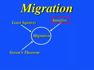
Migration Intuitive Least Squares Green’s Theorem Migration
ZO Migration Smear Reflections along Fat Circles xx + T xx o 2-way time x Thickness = c*T /2 x o 2 2 (x-x ) + y = xx c/2 d(x , ) Where did reflections come from?
ZO Migration Smear Reflections along Fat Circles xx & Sum 1-way time x Hey, that’s our ZO migration formula d(x , )
ZO Migration Smear Reflections along Circles & Sum 1-way time x In-Phase Out-of--Phase d(x , ) xx m(x)=
i xx’ m(x’) x’ reflectivity d = L m e A(x,x’) i ij j j Born Forward Modeling ~ d(x) = g(x|x’)
Seismic Inverse Problem 2 Soln: min || Lm-d || -1 T T m = [L L] L d migration waveform inversion T L d Given: d= Lm Find: m(x,y,z)
i Forward Modeling (d = Lo) ZO Depth Migration (m L d) T xx’ xx’ xx’ m(x’) x x’ Fourier Transform reflectivity e x A(x,x’) w 2 ~ d(x, ) d(x) d(x, ) = m(x’) A(x,x’) .. ~ ~ d(x) = g(x|x’) m(x’) ..
Migration Forward Problem: d=Lm Intuitive Least Squares T m=L d Green’s Theorem Japan Sea Example Migration
Kirchhoff Migration Image LSM Image with a Ricker Wavelet (15 Hz) Actual Model LSM Image 0 0 Depth (km) Depth (km) 2 2 0 0 2 2 X (km) X (km)
2D Poststack Data from Japan Sea JAPEX 2D SSP marine data description: Acquired in 1974, Dominant frequency of 15 Hz. 0 TWT (s) 5 20 0 X (km)
LSM vs. Kirchhoff Migration LSM Image Kirchhoff Migration Image 0.7 0.7 Depth (km) Depth (km) 1.9 1.9 4.9 4.9 2.4 2.4 X (km) X (km)
Migration Intuitive Least Squares Green’s Theorem Migration
x obliquity xx’ q x’ x Approx. reflectivity ~ 3. ZO migration matrix-vec: m=L d T Compensates for Illumination footprint and poor illumination cos q -1 T T 4. LSM ZO migration matrix-vec: m=[L L] L d Summary .. m(x’) d(x, ) = 1. ZO migration: A(x,x’) 2. ZO migration assumptions: Single scattering data 5. ZO migration smears an event along appropriate doughnut
Find: m that minimizes sum of squared residuals r = L m - d j i ij j i (r ,r) = ([Lm-d],[Lm-d]) = 2 m L Lm -2 m Ld (r ,r) = m L Lm -2m Ld-d d = 0 d d d i i dm i dm dm L Lm = Ld Recall: Lm=d Least Squares For all i Normal equations
j i i j i i j i Recall: (u,u) = u* u i i Recall: (v,Lu) = v* ( L u ) i ij j [ L v* ]u = j ij i = [ L* v ]* u ij i j So adjoint of L is L L* ij Dot Products and Adjoint Operators