Geo-neutrinos
660 likes | 838 Vues
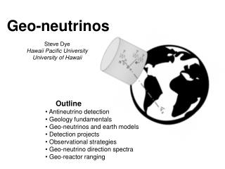
Geo-neutrinos. Steve Dye Hawaii Pacific University University of Hawaii. Outline Antineutrino detection Geology fundamentals Geo-neutrinos and earth models Detection projects Observational strategies Geo-neutrino direction spectra Geo-reactor ranging. Antineutrino Detection.

Geo-neutrinos
E N D
Presentation Transcript
Geo-neutrinos Steve Dye Hawaii Pacific University University of Hawaii • Outline • Antineutrino detection • Geology fundamentals • Geo-neutrinos and earth models • Detection projects • Observational strategies • Geo-neutrino direction spectra • Geo-reactor ranging
Antineutrino Detection Antineutrino (Eν>1.8 MeV) interacts with free proton γ n p+ p+ νe γ e+ e- γ PMTsmeasure position and amount of deposited energy Delayed event deposits energy of 2.2 MeV Scintillating oil Prompt event deposits energy of Eν-0.8 MeV
Reines and Cowan Savannah River At Hanford, Washington Over 5 decades of antineutrino detection Reines, F., Rev. Mod. Phys. 68 (1996) 317-327.
Earth Origin H O C N Solar photosphere (atoms Si = 1E6) B Li C1 carbonaceous chondrite (atoms Si = 1E6) Planets form from solar nebula Carbonaceous chondrite Formation time ~10-100 Ma
Standard Model of Earth Bulk earth (chondrite) = Primitive mantle (komatiite) + Core (Fe/Ni) Primitive mantle (Bulk Silicate Earth) = Mantle + Crust
Earth Structure- Geophysics Detailed seismological description: Preliminary Reference Earth Model (PREM) A.M. Dziewonski, D.L. Anderson, Phys. Earth Planet Inter. 25 (1981) 297. Seismology defines earth structure
U, Th, K principal heat-producing elements 20±4 TW Earth Composition- Geochemistry What are amount and distribution of U, Th, K in crust and mantle? Bulk Silicate Earth model: ~1/2 of U, Th, K in crust ~1/2 of U, Th, K in mantle ~no U, Th, K in core
Earth Heat- Geodynamics Surface Heat Flow Measurement Sites Heat flow probe- thermal conductivity, dT/dx Heat conduction- q = -k dT/dx Surface heat flow interpretations: Jaupart et al. (2008) Aq=46±3TW Hofmeister and Criss (2004) Aq=33±1TW
Surface Heat Flow Radiogenic Heat Production 238U 40K 232Th Surface heat flow interpretations: Jaupart et al. (2008) Aq=46±3TW Hofmeister and Criss (2004) Aq=33±1TW Radiogenic heat estimate: (hU≈ hTh≈ ⅜hK) McDonough and Sun (1995) Mh=20±4TW U = Mh/Aq U = 0.43±0.09 U = 0.61±0.12 ∂T/∂t = (Mh-Aq)/MC ∂T/∂t = (-26±5)/MC ∂T/∂t = (-13±4)/MC Thermal Earth: MC(∂T/∂t) = Mh - Aq Radiogenic heat estimate dominates uncertainty in Urey ratio and cooling rate calculations
Terrestrial Antineutrinos 238U 232Th νe+ p+→ n + e+ 1.8 MeV Energy Threshold 1α, 1β 1α, 1β 238U 232Th 40K 234Pa 228Ac 2.3 MeV 2.1 MeV 5α, 2β 4α, 2β 214Bi 212Bi νe νe νe νe 3.3 MeV 2.3 MeV 2α, 3β 1α, 1β 206Pb 40K 40Ca 208Pb Terrestrial antineutrinos from uranium and thorium are detectable 1β
Crust thickness & density Bassin, C., Laske, G. and Masters, G. (2000) 7 layers in 16,200 tiles each 2° x 2° 360 crust types!!! U & Th concentrations Rudnick, R.L. and Fountain, D.M. (1995) a(U) 2.8, 1.6, 0.2 ppm a(Th) 10.7, 6.1, 1.2 ppm Geo-neutrinos – Crust Assume geo-neutrino flux scales with heat production: requires detailed study Constrain models with 15% measurements
Geo-neutrinos – Mantle Mantle model typically radial-symmetric } ΔH ~ 10% but Δφ ~ 25% Constrain models with ~10% measurements
Earth Heat Turcotte-Paul-White 2001 Jaupart-Labrosse-Mareschal 2007 Tolstikhin-Hofmann 2005 Surface heat flow does not constrain radiogenic heat production Shaw 1986 Taylor-McLennan 1985
Mantle Heat vs Rate Jaupart-Labrosse-Mareschal 2007 Tension between some models and geo-dynamics
Terrestrial Antineutrino Reference Model CRUST 2.0 w/ PREM interior U, Th, K concentrations in crust and upper mantle from average of published values Lower mantle constrained by mass balance and- 232Th/238U = 3.9 ; 40K/238U = 1.36 F. Mantovani et al., Phys. Rev. D 69 (2004) 013001.
Reactor Antineutrinos- Background Spectra overlap Neutrino Energy • Reactor flux: • can not be eliminated • grows with each new reactor • minimize by distance
Geo-neutrino Detector Parameters Reference model rates corrected for new νosc parameters
Reactor Spectra at Detection Sites Gran Sasso Kamioka Sudbury Homestake Baksan Pyhasalmi 201 reactors worldwide with total power 1.064 TW
Borexino- in Italy Primary Goal νe+ e- →νe+ e- Solar neutrino- electron scattering • operating since 5/16/07 • 300 tonnes LS • 2200 PMTs • ~30% PC coverage No terrestrial antineutrino results yet
KamLAND- in Japan Primary Goal νe+p→ n + e+ Reactor antineutrino inverse beta • operating since 3/9/02 • 1000 tonnes LS • 1879 PMTs Terrestrial antineutrino results 2004, 2008 2.44x1032 proton-yr
Prompt Event Energy Spectrum arXiv:0801.4589v2 [hep-ex] 5 Feb 2008 KamLAND Geo-neutrino Results Large background limits sensitivity to geo-neutrinos No evidence yet for U-series geo-neutrinos Best fit to data for Th/U=3.9 gives 73±27 (2.7σ) events, consistent with reference model, a precision of 37%
KamLAND U & Th Flux Turcotte-Paul-White 2001 Tolstikhin-Hofmann 2005 Shaw 1986 Ref (Mantovani et al. 2004) Taylor-McLennan 1985 Ref KamLAND flux measurement does not constrain models
Future Terrestrial Antineutrino Results LENA Baksan Hanohano
Predicted Antineutrino Source Fractions Future detector sites better for terrestrial antineutrino flux measurements
Fractional Uncertainty: Crust, Mantle Rates Rate of antineutrino events: Uncertainties Fractional uncertainties Background subtraction requires model assumption
Background-subtracted Crust Rate Precision KamLAND • Mantle rate m=8.9 TNU • Exposure error σe=0.03 • Reactor error σr=0.03 • Oscillation error σo=0.03 • Mantle error σm=0.20 • Solid- 1.0c • Dash- 1.2c • Dots- 0.8c Borexino SNO+ SNO+ has potential for 20% measurement of background-subtracted crust rate in 3-6 years
Crust Rate…future 2.5-kt DUSEL • Mantle rate m=8.9 TNU • Exposure error σe=0.03 • Reactor error σr=0.03 • Oscillation error σo=0.03 • Mantle error σm=0.20 • Solid- 1.0c • Dash- 1.2c • Dots- 0.8c 5-kt Baksan 50-kt LENA All have potential for 10% measurement of background-subtracted crust rate
Detection parameters: n2 = c2 + m + r2 n1 = c1 + m + r1 c2– c1 = (n2 – r2) – (n1 – r1) rates: Compare measurements at two sites: exposure: σr ,σe ,σo errors: Fractional Uncertainty: Crustal Rate Difference Insensitive to mantle model Construct fractional uncertainty in crustal rate difference: Maximize Δn , ε ; Minimize r, σr , σe , σo
KamLAND – Borexino – SNO+ KamLAND - Borexino • KamLAND – Borexino • ~250% • KamLAND – SNO+ • ~100% • Borexino – SNO+ • ~80% KamLAND - SNO+ Detectors capable of geo-neutrino observation, which are existing or under construction, are not able to resolve crustal models independent of BSE Borexino - SNO+ Solid σr =σe =σo =0.03; Dots σr =σe =σo=0.01; Dash σr =σe =σo =0.05
Continental vs. Oceanic Hanohano – KamLAND Hanohano – Borexino Hanohano – SNO+ • Hanohano – KamLAND • ~60% • Hanohano – Borexino • ~20% • Hanohano – SNO+ • ~16% Combined continental and oceanic geo-neutrino observation can constrain crustal models independently of BSE only after very long time Solid σr =σe =σo =0.03; Dots σr =σe =σo=0.01; Dash σr =σe =σo =0.05
Continental vs. Oceanic – Future HH – 2.5-kt DUSEL HH – 5-kt Baksan HH – 50-kt LENA • Hanohano – 2.5-kt DUSEL • ~8% • Hanohano – 5-kt Baksan • ~8% • Hanohano – 50-kt LENA • ~9% Combined continental and oceanic geo-neutrino observation can constrain crustal models independently of BSE in reasonable time Solid σr =σe =σo =0.03; Dots σr =σe =σo=0.01; Dash σr =σe =σo =0.05
Background-subtracted mantle rate precision • Crust rate c=3.6 TNU • Crust error σc=0.20 Exposure at mid-oceanic site helps constrain mantle models but does not determine U and Th distribution Solid σr =σe =σo =0.03; Dots σr =σe =σo=0.01; Dash σr =σe =σo =0.05
Boundaries in a 1-Dimensional Mantle Transition Zone 63.5° CMB 33.1° Re ρ Core Mantle Nadir angle cos(θ) = (Re2-ρ2)1/2/Re Re= 6371 km ρCMB= 3480 km cos(θCMB) = 0.84 ρTZ=5701 km cos(θTZ) = 0.45 Symmetry enhances signal
Resolving Mantle Models KT97 TZ CMB TKH06 Layered Mantle Convection Outer core Whole Mantle Convection Angular distribution of antineutrinos identifies mantle layers with different U, Th concentrations
Geo-neutrino Directions- Crust Need to add site-specific crustal signal to model-dependent mantle signal Could the crust and mantle be separately resolved?
Preliminary Angular Resolution Study KT97 TKH06 99.7% CL 95.5% CL 68.3% CL Compare red/blue ratios Calculate exposure to resolve Crust signal mostly here Resolution of mantle models depends on angular resolution
Measuring Antineutrino Direction Reconstructed event direction • Interaction kinematics • Neutron absorption • Position resolution • Scintillator properties Δθ Delayed n capture Δθ Neutron Emission Angle θn νe Neutrino direction Prompt e+ Neutron Kinetic Energy (keV) • Can we build a nuebar telescope? • Good for geology, DSNB search • Would be an interesting study
Geo-neutrino Conclusions • Remote sensing of main heat-producing elements- U, Th • Demonstrated by KamLAND • Detected flux depends on quantity and distribution of U, Th • >3 km water equivalent & far from reactors • Disentangle contributions from crust and mantle with • Continental AND Oceanic observatories • 2.5-kt DUSEL (40M$) and 10-kt Hanohano (>100M$) • Distribution of U, Th in mantle may require direction • Promising developments in progress
A Natural Fission Reactor Predicted by P.K. Kuroda, J. Chem. Phys. 25, 781 (1956). Discovered at Oklo in west Africa G.A. Cowan, Sci. Am. 235, 36 (1976). • 235U/238U ~0.03 (~4 x present) 2 Gy ago • Water concentrates deposit & moderates n • Reactor released ~15 GW-yr of energy over • few 105 yr
Deep-Earth Geo-reactor Models • Proposed at 3 depths w/ loosely defined • power output sufficient to explain: • surface heat flow > radiogenic heat • 33-46 TW > ~20 TW • 3He/4He OIB>MORB • tritium fission product- 3H→3He+β-+ν r=3480 km Core-Mantle Boundary P~5TW R.J. de Meijer & W. van Westrenen S. Afr. J. Sci. 104, 111 (2008) Inner Core Boundary P~20-30 TW V.D. Rusov et al., J. Geophys. Res. 112, B09203 (2007) r=1222 km Earth Center P~3-10 TW J.M. Herndon, Proc. Nat. Acad. Sci. 93, 646 (1996) Deep-earth Geo-reactor: Hypothetical and very speculative Possible and not ruled out
Experimental Constraint 55 Japanese nuclear power reactor units - Nuclear plant KamLAND exposure 2.44x1032p+-yr and solar neutrino data set upper limit to power of earth-centered geo-reactor P < 6.2 TW (90% C.L.) Abe et al., PRL 100, 221803 (2008)
More Sensitive Search Possible Oceanic antineutrino observatory operating far from reactors in deep ocean Signal/Background ~0.8/TW 8.5x1032 p+-yr exposure sets P < 0.5 TW at >95% C.L. Or measure power to ~10% if P~ few TW at earth center Dye et al., EMP 99, 241 (2006)
Uncertainties- Power vs Location What if geo-reactor not earth-centered? Models suggest 3 possible deep-earth locations: Earth center Inner core boundary Core-mantle boundary Could consider antineutrino direction measurement Excellent recent progress at RCNS although technology not fully available …or use neutrino oscillation pattern to make the map KamLAND power limit translates to 1.3 – 15 TW allowing geo-reactor position along diameter through core Locating geo-reactor source position would lead to more precise power estimate and discriminate geo-reactor models
Reactor antineutrino energy spectrum Earth center d=6370 km δE=0 Core-mantle d=2890 km δE=0 Distortion of Energy Spectrum Reactor spectrum approximated Mixing parameters from global solar + reactor fit eV2 Abe et al., PRL 100, 221803 (2008)
δE=6%√E δE=3%√E 6370 km 5150 km 2890 km Energy Resolution Idealized energy spectra: TW-1033p+-yr Benchmark: KamLAND visible energy resolution δE/E=6.5%/√E Visible energy related to antineutrino energy • Visible energy resolution • determined by scintillation • light collection: • Photocathode coverage • Photocathode QE • Scintillation light output Distortions well preserved with 3%√E energy resolution
Brighter Scintillating Oil Increase light output with LAB-based scintillating oil x ~1.7 (M. Chen 2006) Increase photocathode coverage to SNO-like (55%) x ~1.6 (B. Aharmin et al. 2007) Increase PC quantum efficiency x ~1.6 (R. Mirzoyan et al. 2006) Improving Energy Resolution Benchmark- KamLAND at ~6% Goal- Increase light collection x4 to achieve 3% 3%√E possible
For each event in the spectrum Independent Distance ~150 km Rayleigh Power Estimates Spectral Significance amplitude modulation Introduced by Lord Rayleigh to study directions of pigeon flight Used to test for periodicity of light curves in astronomy Test significance of spectrum at distances L=500-8000 km Use Rayleigh Power to estimate significance of spectral distortions Distance limitations: spectrum must modulate, Lind is minimum; modulations must be resolved, energy resolution sets maximum
Rayleigh Power Distributions Idealized energy spectra: TW-1033p+-yr δE=6%√E δE=3%√E δE=6%√E δE=3%√E 6370 km 5150 km 2890 km Oversampled x10 Measuring Distance to Reactor Power peaks at correct distance FWHM ~1000 km
Resolving Distances to Multiple Sources • Idealized energy spectrum with • δE=3%√E from TW-1033p+-yrexposure • to sources at: • CMB • Inner core boundary- near • Earth center • Inner core boundary- far Rayleigh power distribution resolves discrete sources at different distances separated by > ~500 km Method capable of finding discrete sources at different distances