MR Image Formation
MR Image Formation. FMRI Graduate Course (NBIO 381, PSY 362) Dr. Scott Huettel, Course Director . Introductory Exercise. Write down the major steps involved in the generation of MR signal Just write an outline, not an essay Note what scanner component contributes to each step.

MR Image Formation
E N D
Presentation Transcript
MR Image Formation FMRI Graduate Course (NBIO 381, PSY 362) Dr. Scott Huettel, Course Director FMRI – Week 3 – Image Formation Scott Huettel, Duke University
Introductory Exercise • Write down the major steps involved in the generation of MR signal • Just write an outline, not an essay • Note what scanner component contributes to each step FMRI – Week 3 – Image Formation Scott Huettel, Duke University
Generation of MR Signal FMRI – Week 3 – Image Formation Scott Huettel, Duke University
T1 T2 FMRI – Week 3 – Image Formation Scott Huettel, Duke University
Relaxation Times and Rates • Net magnetization changes in an exponential fashion • Constant rate (R) for a given tissue type in a given magnetic field • R = 1/T, leading to equations like e–Rt • T1 (recovery): Relaxation of Mback to alignment with B0 • Usually 500-1000 ms in the brain (lengthens with bigger B0) • T2 (decay): Loss of transverse magnetization over a microscopic region ( 5-10 micron size) • Usually 50-100 ms in the brain (shortens with bigger B0) • T2*: Overall decay of the observable RF signal over a macroscopic region (millimeter size) • Usually about half of T2 in the brain (i.e., faster relaxation) FMRI – Week 3 – Image Formation Scott Huettel, Duke University
T1 Recovery FMRI – Week 3 – Image Formation Scott Huettel, Duke University
T2 Decay FMRI – Week 3 – Image Formation Scott Huettel, Duke University
T1 and T2 parameters By selecting appropriate pulse sequence parameters (Week 4’s lecture), images can be made sensitive to tissue differences in T1, T2, or a combination. FMRI – Week 3 – Image Formation Scott Huettel, Duke University
I FMRI – Week 3 – Image Formation Scott Huettel, Duke University
FMRI – Week 3 – Image Formation Scott Huettel, Duke University
Gradients change the Strength, not Direction of the Magnetic Field FMRI – Week 3 – Image Formation Scott Huettel, Duke University
Parts of 2D Image Formation • Slice selection • Linear z-gradient • Tailored excitation pulse • Spatial encoding within the slice • Frequency encoding • Phase encoding FMRI – Week 3 – Image Formation Scott Huettel, Duke University
Slice Selection FMRI – Week 3 – Image Formation Scott Huettel, Duke University
FMRI – Week 3 – Image Formation Scott Huettel, Duke University
Linear z-gradient FMRI – Week 3 – Image Formation Scott Huettel, Duke University
Why can’t we just use an excitation pulse of a single frequency? FMRI – Week 3 – Image Formation Scott Huettel, Duke University
Selecting a Band of Frequencies FMRI – Week 3 – Image Formation Scott Huettel, Duke University
Choosing a Slice FMRI – Week 3 – Image Formation Scott Huettel, Duke University
Changing Slice Thickness FMRI – Week 3 – Image Formation Scott Huettel, Duke University
Changing Slice Location (Note: manipulating gradient is simpler than changing slice bandwidth.) FMRI – Week 3 – Image Formation Scott Huettel, Duke University
… 13 12 Interleaved Slice Acquisition … 3 2 1 FMRI – Week 3 – Image Formation Scott Huettel, Duke University
FMRI – Week 3 – Image Formation Scott Huettel, Duke University
Spatial Encoding FMRI – Week 3 – Image Formation Scott Huettel, Duke University
How not to do spatial encoding… FMRI – Week 3 – Image Formation Scott Huettel, Duke University
… a better approach FMRI – Week 3 – Image Formation Scott Huettel, Duke University
Temporal Signal = Combination of Frequencies FMRI – Week 3 – Image Formation Scott Huettel, Duke University
Effects of Gradients on Phase FMRI – Week 3 – Image Formation Scott Huettel, Duke University
Core Concept:k-space coordinate = Integral of Gradient Waveform FMRI – Week 3 – Image Formation Scott Huettel, Duke University
k-space Image space ky y kx x Acquired Data Final Image Fourier Transform Inverse Fourier Transform FMRI – Week 3 – Image Formation Scott Huettel, Duke University
Spatial Image = Combination of Spatial Frequencies FMRI – Week 3 – Image Formation Scott Huettel, Duke University
k Space FMRI – Week 3 – Image Formation Scott Huettel, Duke University
Image space and k space FMRI – Week 3 – Image Formation Scott Huettel, Duke University
Parts of k space FMRI – Week 3 – Image Formation Scott Huettel, Duke University
So, we know that two gradients are necessary for encoding information in a two-dimensional image? What would happen if we turned on both gradients simultaneously? FMRI – Week 3 – Image Formation Scott Huettel, Duke University
Frequency Encoding • During readout (or data acquisition, DAQ) • Uses gradient perpendicular to slice-selection gradient • Signal is sampled & digitized about once every few microseconds • Readout window ranges from 5–100 milliseconds • Why not longer than this? • Fourier transform converts signal S(t) into frequency components S(f) FMRI – Week 3 – Image Formation Scott Huettel, Duke University
Phase Encoding • Apply a gradient perpendicular to both slice and frequency gradients • The phase of Mxy (its angle in the xy-plane) signal depends on that gradient • Fourier transform measures phase of each S(f) component of S(t) • By collecting data with many different amounts of phase encoding strength, we can assign each S(f) to spatial locations in 3D FMRI – Week 3 – Image Formation Scott Huettel, Duke University
FMRI – Week 3 – Image Formation Scott Huettel, Duke University
Echo-Planar Imaging (EPI) FMRI – Week 3 – Image Formation Scott Huettel, Duke University
Sampling in k-space K Dk FOV FOV = 1/Dk, Dx = 1/K FMRI – Week 3 – Image Formation Scott Huettel, Duke University
Problems in Image Formation FMRI – Week 3 – Image Formation Scott Huettel, Duke University
Magnetic Field Inhomogeneity FMRI – Week 3 – Image Formation Scott Huettel, Duke University
Gradient Problems FMRI – Week 3 – Image Formation Scott Huettel, Duke University