Download
1 / 39
430 likes | 821 Vues
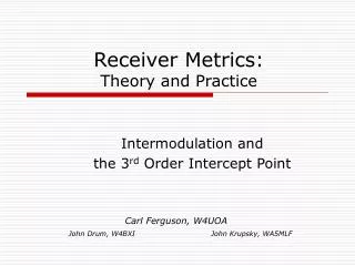
Receiver Metrics: Theory and Practice. Intermodulation and the 3 rd Order Intercept Point. Carl Ferguson, W4UOA. John Drum, W4BXI John Krupsky, WA5MLF. Recent Advertisement. Example Receiver Types & Specs.

E N D
Receiver Metrics:Theory and Practice Intermodulation and the 3rd Order Intercept Point Carl Ferguson, W4UOA John Drum, W4BXI John Krupsky, WA5MLF
Example Receiver Types & Specs • A DC to 30 GHz broadband amplifier using AlGaAs-GaAs heterojunction bipolar transistor (HBT) technology. 7.8 dB gain, IP3=23.9 dBm (ref IEEE Microwave and Guided Wave Letters, Aug 1991) • Monolithic SPDT X-band PIN diode switch. Insertion loss of 0.89 dB, off-isolation >35 dB at 10 GHz, IP3=29.6 dBm. (ref IEEE Microwave and Guided Wave Letters, Oct 1993) • A 44-GHz monolithic microwave integrated circuit (MMIC) amplifier based on InP HBT technology. Gain as high as 7.6 dB, peak IP3=34 dBm. (ref IEEE Journal of Solid-State Circuits, Sep 1999) • PIN photodetectors for RF optical fiber links. Measurement of IP3=27 dBm using a four laser heterodyne system. (ref IEEE Photonics Technology Letters, Apr 2000)
Questions on the Table • What is intermodulation distortion? • What is the 3rd order intercept point? • What do these characteristics mean in practice?
Linear Gain Linear gain in a circuit is normally represented by a straight line. The scale on the Input and Output axis reflect the gain through the circuit. In this example, a gain of 2:1. However, all RF & IF circuits are inherently nonlinear.
Gain and the Compression Point At low input levels, receiver RF and IF stage gain will be generally linear—approaching a level called the small-signal asymptotic value. But as the input level increases, gain through the stage becomes increasingly nonlinear. When the gain falls n dB below the small-signal asymptotic value, it has said to have reached its compression point (CP). The compression point, stated in dB, is frequently given as either 1 dBor 3 dB below the small-signal asymptotic value. Output CP Input
Nonlinearity and Intermodulation Distortion • Nonlinearity in RF and IF circuits leads to two undesirable outcomes: harmonics and intermodulation distortion. • Harmonics in and of themselves are not particularly troublesome. • For example, if we are listening to a QSO on 7.230 MHz, the second harmonic, 14.460 MHz is well outside the RF passband. • However, when the harmonics mix with each other and other signals in the circuit, undesirable and troublesome intermodulation products can occur.
Intermodulation Distortion Products: An Example f1 f2 2f1- f2 2f2- f1 3f2- 2f1 3f1- 2f2 MHz
Why it is called 3rd order Token math slides The performance of an ideal amplifier can be represented by the transfer function: An amplifier with some distortion due to nonlinearities can be expressed by a transfer function in the form of a power series expansion: An input signal with two frequencies 1 and 2may be shown as: The first order term gives the fundamental products The second order term determines the second order products: DC terms 2nd harmonic terms 2nd order IMD terms
Why it is called 3rd order (cont’d) The third order term determines the third order products: Fundamental frequency terms 3rd harmonic terms 3rd order IMD terms – The troublemakers
Third Order Intermodulation Products • The 3rd order products will be the largest (loudest) of the intermodulation products. • As a general rule, the 3rd order products will increase (grow) 3-times faster than the fundamental signal (the signal of interest). However, recent lab studies have revealed that this relation can vary from receiver to receiver.
Intercept Point 3 (IP3): A Measure of Merit Our graph illustrates that the 3rd order intercept point is defined by the intersection of two hypothetical lines. Each line is an extension of a linear gain figure: first of the signal of interest; and second, of the 3rd order intermodulation distortion product—from which IP3 gets its name. While there are several ways that IP3 can be located, you will note that of the several illustrated here, they all fall in the same general area. The larger the value of IP3, the less likely the receiver will be adversely affected by 3rd order intermodulation products. More on this later.
Dynamic Range:A Measure of Merit • The ratio of the smallest usable signal to the largest tolerable signal. • The amplitude range over which a mixer can operate without degradation of performance. • Noise should determine the lower limit of a receiver’s dynamic range. • The lower limit may be defined by the signal-to-noise ratio of a desired signal at its output. This measure is generally favored because of its empirical nature—it can be easily calculated. • However, the lower limit can be set by the MDS—a some what more qualitative measure. • The upper limit is normally set by either noise or distortion. Source: QEX, July/August, 2002.
Lb Lower bound The lower bound is Defined as a signal of interest 3 dB greater than the noise floor. Upper bound Ub The upper bound is set by the compression point of the desired (on-channel) signal. Compression-Free Dynamic Range Compression-FreeDynamic Range Lb Ub
Upper bound Ub Spurious-FreeDynamic Range Lb The upper bound is set by the 3rd order IMD equal to theMDS. Ub Spurious-Free Dynamic Range Lb Lower bound The lower bound is defined as a signal of interest 3 dB greater than the noise floor.
Upper bound Ub The upper bound is set by the 3rd order IMD equal to theMDS. Spurious-Free Dynamic Range Why is it important to have a wide dynamic range? Notice below that an input signal of -110 dBm will produce 20 dB output in our signal of interest. To achieve 20 dB output in the third order product, the off channel test signals f1 and f2 must be 80 dB (110 dBm – 30 dBm) greater than our signal of interest. An unlikely occurrence except in unique circumstance. Lb Lower bound The lower bound is Defined as a signal of interest 3 dB greater than the noise floor. Spurious-FreeDynamic Range Lb Ub
Spurious-Free Dynamic Range FT-1000 IPO Button Normally, the front-end FET RF amplifiers provide maximum sensitivity for weak signals. During typical conditions on lower frequencies (such as strong overloading from signals on adjacent frequencies), the RF amplifiers can be bypassed by pressing the [IPO] button so the green LED is on. This improves the dynamic range and IMD (intermodulation distortion) characteristics of the receiver, at a slight reduction of sensitivity. On frequencies below about 10 MHz, you generally will want to keep the [IPO] button engaged, as the preamplifiers are usually not needed at these frequencies.
Example performance data From ARRL test reports in QST magazine(at 14 MHz w preamp off)
Automated IP3 Testing • An approach for built-in self testing of RF Integrated Circuits was reported by the Department of Electrical and Computer Engineering at Auburn University. • The goal is to reduce the cost of RF testing on manufactured RFICs (operating in the 2-5 GHz range). The design would provide the ability “to detect faults and to assist in characterization and calibration during manufacturing and field testing”. • The proposed design makes use of Direct Digital Synthesis (DDS) test pattern generator and analyzer circuitry on the chip to perform a 2-tone test and analyze the results. • The prototype design was found to provide accurate results for IP3 values below 30 dBm and is thought to underestimate IP3 values above that.
A Few Final Comments: Sensitivity and Blocking • While a receiver’s ability to handle 3rd order intermodulation products is important—its sensitivity and ability to handle strong adjacent signals is of equal and maybe even greater importance. • We obviously want our receiver to have a very low noise figure—able to hear the weakest of signals. And, we recognize that our RF and IF amplifiers can not handle infinitely large signals—at some point the amplifier will reach its compression point. • What happens when large adjacent signals capture the front-end of our receiver?
Sensitivity and Blocking • Blocking happens when a large off channel signal causes the front-end RF amplifier to be driven to its compression point. • As a result all other signals are lost (blocked). • This condition is frequently called de-sensing—the sensitivity of the receiver is reduced. • Blocking is generally specified as the level of the unwanted signal at a given offset. • Original testing used a wide offset—typically 20 kHz. More recently, recognizing our crowded band conditions and the narrow spacing of CW and other digital modes, most testing today is done with close spacing of 2 kHz.
Sensitivity and Blocking • A good receiver design must find a balance between sensitivity and strong signal handling capability. And while the AGC in most receivers will attenuate large signals, large off channel signals can dramatically reduce a receiver’s sensitivity. • For an excellent presentation on this subject, we refer you tohttp://www.sherwood-engineering.comorhttp://www.NC0B.com
Summary • I hope we’ve answered a few of your questions about: • intermodulation distortion products; • the 3rd order intercept point; • dynamic range; and • maybe stimulated your interest in learning even more about receiver performance.
References • R. Sherwood, NC0B, “Roofing Filters, Transmitted IMD & Receiver Performance”, Presentation to Boulder, Colorado Amateur Radio Club, February 2008, http://www.sherweng.com/ • M. Tracy, KC1SX, “Changes to ARRL Receiver Tests”, QST, October 2007, pp. 70-71 • J. Hallas, W1ZR, “Keeping the Lid on with a Roofing Filter”, QST, October 2007, pp. 57-58 • D. Newkirk, AB2WH, “ICOM IC-9500 Communications Receiver”, Product Review, QST, January 2008, pp.69-73 • B. Prior, N7RR, “First Look: Elecraft K3 HF/6 Meter Transceiver”, Product Review, QST, April 2008, pp. 41-45 • D. Smith, KF6DX, “Improved Dynamic Range Testing”, QEX , Jul/Aug 2002, pp. 46-52 • “Mixers, Modulators and Demodulators”, The ARRL Handbook for Radio Amateurs, 1998, Chapter 15 pp. 15.18-15.21 • U. Rohde, KA2WEU, “Testing and Calculating Intermodulation Distortion in Receivers”, QEX, July 1994, pp 3-4 • K. Kundert, “Accurate and Rapid Measurement of IP2 and IP3”, The Designer’s Guide Community, May 2006, http://www.designers-guide.org • S. Rumley, KI6QP, “A Precision Two-Tone RF Generator for IMD Measurements”, QEX, April 1995, pp. 6-12 • “Radio receiver strong signal response”, Adrio Communications Ltd, http://www.radio-electronics.com/info/receivers/overload/strong_signal_specs.php • M. Ellis, “Introduction to Mixers”, 1999, http://michaelgellis.tripod.com/mixersin.html • “High Dynamic Range Receiver Parameters”, Tech-notes, Vol.7, No. 2, Watkins-Johnson Company, March/April 1980 • “Third Order Intercept Point Versus Sensitivity”, Application Note No. 1.01, Dynamic Sciences International, Inc., May 2005, http://www.dynamicsciences.com/client/show_product/7 • “Theory of Intermodulation Distortion Measurement”, Application Note 5C-043, Maury Microwave Corporation, July 1999, http://www.maurymw.com/support/pdfs/5C-043.pdf • Foster Dai, et al., “Automatic Linearity (IP3) Test with Built-In Pattern Generator and Analyzer”, Proc. IEEE International Test Conf., pp. 271-280, 2004, http://www.eng.auburn.edu/~strouce/class/bist/ITC04ip3.pdf
An early reference Intercept point and undesired responses Sagers, R.C. Motorola, Inc., Fort Worth, Texas; This paper appears in: Vehicular Technology Conference, 1982. 32nd IEEEPublication Date: 23-26 May 1982Volume: 32, On page(s): 219- 230Posted online: 2006-06-19 10:22:27.0 AbstractThis paper presents a method for using the concept of intercept point to calculate the undesired-response rejection ratio of a single stage. Single stages may be cascaded together to form a system and the undesired response rejection ratio of the system may be found using a procedure similar to cascaded noise figure. When applied to receiver system design, this method allows easy calculation of such undesired receiver responses as intermodulation distortion and spurious responses.
A earlier reference Two-Tone Nonlinearity Testing - The Intercept Point Fulton, F.F.This paper appears in: Microwave Symposium Digest, G-MTT InternationalPublication Date: Jun 1973Volume: 73 , On page(s): 112 - 112 Posted online: 2003-01-06 17:17:01.0 AbstractWhen a nonlinearity is modeled as memoryless with a three-term power series, a convenient way of expressing the characteristics is by the use of intercept points. An intercept point is the output power level at which the fundamental tone and the distortion tone have equal amplitudes. For many practical system problems, specification of an intercept point permits very quick calculation of distortion tone levels; in particular, given two equal amplitude fundamental tones at similar frequencies, the adjacent third order distortion product is down from a fundamental by twice the number of decibels that the fundamental is down from the third order intercept point. Even more simply, the second order distortion is down from a fundamental by an amount equal to the number of decibels that the fundamental is down from the appropriate intercept point.