Download
1 / 47
470 likes | 483 Vues
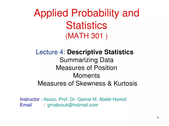
Applied Probability and Statistics ( MATH 301 ) Lecture 4: Descriptive Statistics Summarizing Data Measures of Position Moments Measures of Skewness & Kurtosis. Instructor : Assoc. Prof. Dr. Gamal M. Abdel-Hamid Email : gmabrouk@hotmail.com. Objectives.

E N D
Applied Probability and Statistics(MATH 301 )Lecture 4: Descriptive Statistics Summarizing DataMeasures of PositionMoments Measures of Skewness & Kurtosis Instructor : Assoc. Prof. Dr. Gamal M. Abdel-Hamid Email : gmabrouk@hotmail.com
Objectives • At the end of this lecture, we will be able to • Find Measures of Position • Z Score • Quartiles. • Deciles. • Percentiles. • Exploratory Data Analysis: Box Plot • Find Moments • Find Skewness & Kurtosis
Measures of Position In addition to measures of central tendency and measures of variation, there are measures of position or location. These measures include standard scores, percentiles, deciles, and quartiles. They are used to locate the relative position of a data value in the data set. z Score Quartiles, Deciles, Percentiles
z Score z Score(or standard score) the number of standard deviations that a given value x is above or below the mean Interpreting Z Scores Unusual Values Unusual Values Ordinary Values - 3 - 2 - 1 0 1 2 3 Z
Example 1 A student received a grade of 84 on a final examination in Math for which the mean grade was 76 and the standard deviation was 10. He received a grade of 90 on his final examination in Physics for which the mean grade was 82 and the standard deviation was 16. Compare his relative positions on the two tests. Solution Z Math = (84 – 76)/10 = 0.8 Z Physics = (90– 82)/16 = 0.5 The student a Math grade that is 0.8 of the standard deviation above the mean, and a Physics grade that is 0.5 of the standard deviation above the mean, thus the student is relatively standing (relative position) higher in Math.
Sample Percentiles • Sometimes it is important to know below which value a certain percentage of data in a data set lies. • Let p be from [0,1]. The sample 100p percentile is a value such that • 100p % of the data are less than or equal to it, • And 100(1-p)% of the data are greater than or equal to it. • If two values satisfy this condition, then their arithmetic average is taken.
Percentiles 99 Percentiles
Example 2 The frequency distribution for the systolic blood pressure readings (in millimeters of mercury, mm Hg) of 200 randomly selected college students is shown here. Construct a percentile graph.
Solution Once a percentile graph has been constructed, one can find the approximate corresponding percentile ranks for given blood pressure values and find approximate blood pressure values for given percentile ranks.
For example, For a blood pressure reading of 130, the percentile rank is approximately the 70th percentile. If the value that corresponds to the 40th percentile is desired, the 40th percentile corresponds to a value of approximately 118. Thus, if a person has a blood pressure of 118, he or she is at the 40th percentile.
10% 10% 10% 10% 10% 10% 10% 10% 10% 10% D1 D2 D3 D4 D5 D6 D7 D8 D9 Deciles D1, D2, D3, D4, D5, D6, D7, D8, D9 divides ranked data into ten equal parts
Sample Quartiles • The sample 25th, 50th and 75thpercentiles are called the sample 1st , 2nd and 3rdQuartiles, respectively. • As their names suggest they split a data set into 4 parts with roughly equal number of values. • Note: the Second Quartile is simply the median.
Quartiles Q1, Q2, Q3 divides ranked scores into four equal parts 25% 25% 25% 25% Q1 Q2 Q3 (minimum) (maximum) (median)
Exploratory Data Analysis The process of using statistical tools (such as graphs, measures of center, and measures of variation) to investigate the data sets in order to understand their important characteristics
Exploring • Measures of center:mean, median, and mode • Measures of variation: Standard deviation and range • Measures of spread and relative Location: minimum values, maximum value, and quartiles • Unusual values: outliers • Distribution: histograms, stem-leaf plots, and box plots A box plot used for Exploratory Data Analysis
The Five-Number Summary and Boxplots A boxplot can be used to graphically represent the data set. These plots involve five specific values: 1. The lowest value of the data set (i.e., minimum) 2. Q1 3. The median 4. Q3 5. The highest value of the data set (i.e., maximum) These values are called a five-number summary of the data set.
Box Plots • A box plot for a data set is a straight line segment stretching from the smallest to the largest value, drawn on a horizontal axis. • On the line we impose a “box” that starts at Quartile 1 and ends at Quartile 3. • The value of the median = Quartile 2 is indicated by a vertical line. • The value IQR = Q3 - Q1 is called the inter-quartile range of the data. • The data values smaller than Q1 - 1.5 IQR and larger than Q3+1.5 IQR are called outliers and marked by small circles on the horizontal line • The data lying outside the interval [Q1-3IQR,Q3+IQR] are called extreme outliers.
Box plots(Box-and-Whisker Diagram) Reveals the: • center of the data • spread of the data • distribution of the data • presence of outliers Excellent for comparing two or more data sets Box plots: 5 number summary - Minimum - first quartile Q1 - Median (Q2) - third quartile Q3 - Maximum
Box plots Bell-Shaped Uniform Skewed
Example 3 The number of meteorites found in 10 states of the United States is 89, 47, 164, 296, 30, 215, 138, 78, 48, 39. Construct a boxplot for the data. Solution
Data for Box Plotting Parameter Value Minimum 1 1st Quartile 3.5 2nd Quartile 6.5 3rd Quartile 13.5 Maximum 18 IQR 10
Example 6 Solution
This was the end of the first part of our course which is “Descriptive Statistics” • Next week we will start Part two which is “Probability Theory”
Points to Remember • Measures of Central Tendency • The Mode, the Median, the Mean, the Weighted Mean • Measures of Variation • The Range • The Variance – The Standard Deviation. • The Coefficient of Variation • Chebyshev’s Theorem • Measures of Position: Quartiles, Deciles, Percentiles • Exploratory Data Analysis: Box Plot • Moments, Skewness & Kurtosis
The following are the final grades, in a certain course, for 80 students • a) Calculate the range. • b) Construct a frequency and a relative frequency histogram for this data. • c) Draw a cumulative frequency and cumulative relative frequency curve for the data. • d) What is the number of students who received grades less than 75? • e) What is the percentage of students who received grades higher than 85? • f) Calculate the arithmetic mean, median, mode, standard deviation and variance for this frequency distribution. • g) Calculate Pearson's first and second coefficients of skewness and the moment coefficient of skewness. • h) Calculate the moment coefficient of kurtosis.
The number of ATM transactions per day was recorded at 20 locations. The data were: 35, 49, 225, 50, 30, 65, 40, 55, 52, 76, 48, 325, 47, 32, 60, 95, 89, 154, 14, and 70. Find • a. the median number of transactions, • b. the mean number of transactions and • c. the mode of the transactions . • 8. a) By adding 5 to each of the numbers in the set 3, 6, 2, 1, 7, 5, we obtain the set 8, 11, 7, 6, 12, 10. Show that the two sets have the same standard deviation but different means. How are the means related? • b) By multiplying each of the numbers in the set 3, 6, 2, 1, 7, 5, by 2 and then adding 5, we obtain the set 11, 17, 9, 7, 19, 15. What is the relationship between the standard deviations and the means for the two sets? • c) What properties of the mean and standard deviation can be concluded from (a) and (b)?