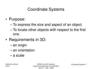
Coordinate Transfer needs
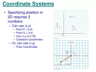
Coordinate Transfer needs. Coastline. NORTH. Cross-shore, y. Alongshore, x. EAST. Instrument Coordinate System. Geographical Coordinate System. Specific Application Coordinate System. Rotation Matrix. (1) Rotation of the axes. (2) Rotation of an Object relative to fixed axes. x.

Coordinate Transfer needs
E N D
Presentation Transcript
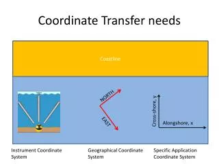
Coordinate Transfer needs Coastline NORTH Cross-shore, y Alongshore, x EAST Instrument Coordinate System Geographical Coordinate System Specific Application Coordinate System
Rotation Matrix • (1) Rotation of the axes. • (2) Rotation of an Object relative to fixed axes x yo θ xo y
Rotate Co-ordinate Axis System(anti-clockwise) y y yo ѳ xo x x
Rotate Object (anti-clockwise)= Rotate Axis (clockwise) y y y1 x1 ѳ x x
Rotate Co-ordinate Axis System y y yo y’ xo x x ѳ ѳ x’
square = 0 0 0 1 1 1 1 0 0 0 Sq2 = 0 0 0.3420 0.9397 1.2817 0.5977 0.9397 -0.3420 0 0 theta = 20 Sq1 = 0 0 -0.3420 0.9397 0.5977 1.2817 0.9397 0.3420 0 0
Example • (1) Make a matlab script that does the rotation (2-d) • (2) Make it a function • (3) Rotate some current data
function X1=rotate_2d(X,a) • % • [m,n]=size(X); • j=1; • if n==2; • X=X'; • j=2; • end • R=[ cos(a) sin(a) • -sin(a) cos(a) ]; • X1=R*X; • if j==2; • X1=X1'; • end • end
a=load(‘L:\787lab\Lecture01\Springmaid_Dec_2005.txt'); yyyy = a(:,1); mo = a(:,2); dd = a(:,3); hh = a(:,4); mi = a(:,5); ss = a(:,6); % u = a(:,7); v = a(:,8); % Time = datenum(yyyy,mo,dd,hh,mi,ss); % U=[u,v]; Uxy=rotate_2d(U,45); ux = Uxy(:,1); uy = Uxy(:,2); % figure subplot(211); plot(Time,u,Time,v); legend('u','v') subplot(212); plot(Time,ux,Time,uy); legend('along','cross') % figure subplot(211); quiver(Time-Time(1),Time*0,u,v); axis equal subplot(212); quiver(Time-Time(1),Time*0,ux,uy); axis equal
Rotations around x-, y- and z- axes • Pitch is up and down like a box lid. • Yaw is left and right like a door on hinges (Heading) • Roll is rotation.
Anticlockwise rotations around x-, y- and z- axes z Roll y α z β Pitch x γ y Yaw x Anticlockwise rotations
3-D Clockwise Rotation cos(β)∙cos(γ) cos(β)∙sin(γ) sin(β) -sin(α)∙sin(β)∙cos(γ)-cos(α)∙sin(g) -sin(α)∙sin(β)∙sin(γ)+cos(α)∙cos(γ) sin(α)∙cos(β) -cos(α)∙sin(β)∙cos(γ)+sin(α)∙sin(g) -cos(α)∙sin(β)∙sin(γ)-sin(α)∙cos(γ) cos(α)∙cos(β)
Rotate 3-D function X1=rotate_3da(X,a,b,g) [m,n]=size(X); j=1; if n==3; X=X'; j=2; end Rx = [ 1 0 0 % Roll 0 cos(a) sin(a) 0 -sin(a) cos(a)]; Ry = [ cos(b) 0 sin(b) % Pitch 0 1 0 -sin(b) 0 cos(b)]; Rz = [ cos(g) sin(g) 0 % Yaw -sin(g) cos(g) 0 0 0 1]; R = Rx*Ry*Rz; % R = [ cos(b)*cos(c), cos(b)*sin(c), sin(b) % - cos(a)*sin(c) - cos(c)*sin(a)*sin(b), cos(a)*cos(c) - sin(a)*sin(b)*sin(c), cos(b)*sin(a) % sin(a)*sin(c) - cos(a)*cos(c)*sin(b), - cos(c)*sin(a) - cos(a)*sin(b)*sin(c), cos(a)*cos(b)] X1=R*X; if j==2; X1=X1'; end end
Exercise 1 • Assume we measure the flow from a boat that pitches and rolls because of the wave motion. • The data are measured in a ship coordinate frame (x,y,z) and the flow is ux=10cm, uy=14cm, uz=5cm. • The heading of the boat is 120deg (Magnetic north) and the magnetic declination is 8degs W and the pitch and roll are 10 and 12degs (anticlockwise) respectively. • What is the true east, north and upward components of the flow? • What is the magnitude of the current? • ( Write a MATLAB function that does the rotation of the vector and corrects for pitch and roll) y X
Working example z Pitch = 10o 8o ux=10 cm / s uy=14 cm / s uz=5 cm/s x 120o z y Rotation around x Rotation around y Rotation around z y Roll = 12o X u= 15.16cm / s v= 9.53 cm / s w= 0.43 cm/s
Converting from an arbitrary (non-orthogonal) coordinate system to a Cartesian coordinate system
Doppler Effect is used to measure velocities along the direction of the acoustic wave propagation (1-D) λ2 λ λ1 c=λ·f c=λ·f c-u=λ·f1 c+u=λ·f2 f1 <f2 f1 =f-Δf f2 =f+Δf c-u=λ·f1 c+u=λ·f2
1-D Doppler current metersPrinciple of operation c : speed of sound in water (depends on T and S) Fo : Frequency of sound transmitted by instrument Df: Doppler shift due to current V V : current speed along the direction of sound propagation Images from: Sontek/YSI
3-D Doppler current metersPrinciple of operation w v V2 V1 c : speed of sound in water (depends on T and S) Fo : Frequency of sound transmitted by instrument Dfi: Doppler shift due to current Vi along beam direction Vi : current speed along the direction of sound propagation (beam i) V3 u Image from: Sontek/YSI
Three Beam to 3-D Phi : Angle of beam from vertical axis Theta: Angle of beam projection to horizontal plane from x-axis (measured, counterclockwise) z phi(1) = AOC1 theta (1)= D1OB1 phi(2) = AOC2 theta (2)= D1OB2 y C2 C1 A B2 B1 x D2 O D1 C3 phi(3) = AOC3 theta (3)= D1OB3 B3
Rotation from arbitrary system to orthogonal coordinate system function T=rotation_matrix(phi,theta) % % phi (in degs) = angle of beam from vertical (z) axis % (phi 1 if the same angle for all beams or % size(phi)=3 if each beam has a different angle % theta (in degs) = angle of beam projection(s) to plane from x, measured counterclockwise % % Vi=T*V and V=inv(T)*Vi % where V=[u,v,w]'; vector of velocities along the x,y,z axis % Vi=[v1,v2,v3]' ; vector of along beam 1, 2 and 3 velocities % % N=length(phi); if N==1; phi=ones(3,1)*phi*pi/180; elseif N==3 phi=phi*pi/180; else error('The Beam angles must be 1 or 3') end phi=phi(:); theta=theta*pi/180; % T(1,:)=[sin(phi(1))*cos(theta(1)) sin(phi(1))*sin(theta(1)) cos(phi(1))]; T(2,:)=[sin(phi(2))*cos(theta(2)+theta(1)) sin(phi(2))*sin(theta(2)+theta(1)) cos(phi(2))]; T(3,:)=[sin(phi(3))*cos(theta(3)+theta(1)) sin(phi(3))*sin(theta(3)+theta(1)) cos(phi(3))];
Two Beam to 3-D phi(1) = AOC1 theta (1)= D1OB1 z phi(2) = 0 theta (2)= 0 y C1 A B1 x O D1 C3 phi(3) = AOC3 theta (3)= D1OB3 B3
Find the mean downstream velocity (Ux) y -10cm/s x 13cm/s 125degs 85degs
Extracting Data from a 2-beam Aquadop • Stations A & B = Nortek Aquadopp • Operating Frequency = 2 MHz • Sampling Frequency = 1 Hz • Number of Samples = 1024 • (~17 minutes) Beam 2 of this Aquadop was inactive Stations C & D = ADV
Beam 3 Beam 2 Original Aquadop Beam Geometry z-axis Beam 1 y-axis V3 V1 x-axis Aquadop Operating Beam Geometry Artificial Aquadop Beam Geometry V2 Beam 3 Beam 3 Beam 2 Beam 1 z-axis Beam 1 y-axis x-axis Extracting Data from a 2-beam Aquadop
Generalized Transformation Matrix V3 V1 V2 v w w = Angle of beam i from vertical z-axis θi= Angle of beam i projection to x-y plane from x-axis, measured counterclockwise
Transformation Matrices Original 3-Beam Configuration Modified 3-Beam Configuration
Calculating Vertical Velocity (artificial Aquadop beam) from Pressure Data MWL z2 w z1 h p
Mean Velocity Error Analysis for Modified Beam Aquadopp <u>n=0 <v>n=0 <u>n=0.22·vn Error in u= <v>n=0.33·vn
Covariance Error Analysis for Modified Beam Aquadopp Noise Contribution
Comparison between data obtained by the three beam solution (red) and data obtained using the wave orbital velocity as beam 2.
Summary • Rotation on a 2-D system • Rotation on a 3-D system • Rotation from an arbitrary to a 3-D system • How to estimate errors due to rotations.