Download

1 / 23
240 likes | 752 Vues
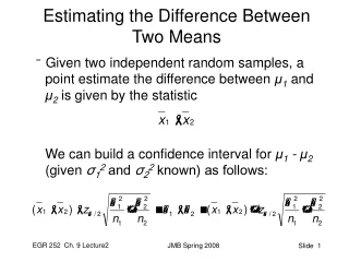
8.2 Testing the Difference Between Means (Small, Independent Samples). Statistics Mrs. Spitz Spring 2009. Objectives/Assignment. How to perform a t-test for the difference between two population means, 1 and 2 using small independent samples. Assignment: pp. 384-388 #1-24 all.

E N D
8.2 Testing the Difference Between Means (Small, Independent Samples) Statistics Mrs. Spitz Spring 2009
Objectives/Assignment • How to perform a t-test for the difference between two population means, 1 and 2 using small independent samples. Assignment: pp. 384-388 #1-24 all
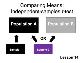
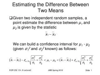
Two Sample t-Test for the Difference Between Means • So, it is impractical and costly to collect samples of 30 or more from each of two populations. What about if both populations have a normal distribution? If so, you can still test the difference between their means. In this section, you will learn how to use a t-test to test the difference between two population means, 1 and 2 using a sample from each population.
Two Sample t-Test for the Difference Between Means • To use a t-Test for small independent samples, the following conditions are necessary: • The samples must be independent, so 1st sample cannot be related to the sample selected from the second population. • Each population must have a normal distribution.
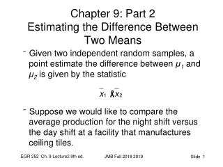
So, the problem meets that criteria, what next? • The sampling distribution for , the difference between he sample means, is a t-distribution with mean The standard error and the degrees of freedom of the sampling distribution depend on whether or not the population variances and are equal.
Pooled Estimate of the Standard Deviation • If the population variances are equal, information from both samples is combined to calculate a pooled estimate of the standard deviation. Pooled estimate of
Pooled Estimate of the Standard Deviation—VARIANCES EQUAL • The standard error for the sampling distribution of is: And d.f. of n1 + n2 - 2
Pooled Estimate of the Standard Deviation-VARIANCES NOT EQUAL • The standard error for the sampling distribution of is: And d.f. smaller of n1 – 1 or n2 - 1
Requirements for z-test • The requirements for the z-test described in 8.1 and the t-test described in this section are compared below: If the sampling distribution for is a t-distribution, you can use a two-sample t-test to test the difference between two populations 1 and 2.
Ex. 1: A Two-Sample t-Test for the Difference Between Means • Consumer Reports tested several types of snow tires to determine how well each performed under winter conditions. When traveling on ice at 15 mph, 10 Firestone Winterfire tires had a mean stopping distance of 51 feet with a standard deviation of 8 feet. The mean stopping distance for 12 Michelin XM+S Alpine tires was 55 feet with a standard deviation of 3 feet. Can you conclude that there is a difference between the stopping distances of the two types of tires? Use = 0.01. Assume the populations are normally distributed and the population variances are NOT equal.
Gather your information . . . • Sample Statistics for Stopping Distances • So now that you have all your relevant data, now go back and figure it out.
Solution Ex. 1 • You want to test whether the mean stopping distances are different. So, the null and alternative hypotheses are: Ho: 1 = 2 and Ha: 1 2 (Claim) Because the variances are NOT equal, and the smaller sample size is 10, use the d.f. = 10 – 1 = 9. Because the test is a two-tailed test with d.f. = 9, and = 0.01, the critical values are?
Solution Ex. 1 • Okay, you got me. . . the critical values are -3.250 and 3.250. The rejection region is t < -3.250 and t > 3.250. The standard error is: Everybody good so far? Questions?
Solution Ex. 1 • Using the t-test, the standardized test statistic is: The graph following shows the location of the critical regions and the standardized test statistic, t.
Solution Ex. 1 • Because t is not in a rejection region, you should fail to reject the null hypothesis. At the 1% level, there is not enough evidence to conclude that the mean stopping distances of the tires are different.
Ex. 2: A Two-Sample t-Test for the Difference Between the Means • A manufacturer claims that the calling range (in miles) of its 900-MHz cordless phone is greater than that of its leading competitor. You perform a study using 14 phones from the manufacturer and 16 similar phones from its competitor. The results are shown on the next slide. At = 0.05, is there enough evidence to support the manufacturer’s claim? Assume the populations are normally distributed and the population variances are equal.
First your sample Statistics for Calling Range • The claim is “the mean range of our cordless phone is greater than the mean range of yours.” So, the null and alternative hypotheses are: Ho: 1 2 and Ha: 1 > 2 (Claim)
Solution Ex. 2 • Because the variances are equal, d.f. = n1 + n2 – 2 = 14 + 16 – 2 = 28 Because the test is a right-tailed test, d.f. = 28 and = 0.05, the critical value is 1.701. The rejecetion is t > 1.701.
Solution Ex. 2 • The standard error is:
Solution Ex. 2 • Using the t-Test, the standardized test statistic is:
Solution Ex. 2 • The graph at the left shows the location of the rejection region and the standardized test statistic, t. Because t is in the rejection region, you should decide to reject the null hypothesis. At the the 5% level, there is enough evidence to support the manufacturer’s claim that its phone has a greater calling range than its competitor’s.