Download
1 / 27
280 likes | 568 Vues
EUROGRAPHICS 2008. A Semi-Lagrangian CIP Fluid Solver Without Dimensional Splitting. 2008.09.12 Doyub Kim Oh-Young Song Hyeong-Seok Ko presented by ho-young Lee. Abstract. USCIP : a new CIP method More stable, more accurate, less amount of computation compared to existing CIP solver

E N D
EUROGRAPHICS 2008 A Semi-Lagrangian CIP Fluid Solver Without Dimensional Splitting 2008.09.12 Doyub Kim Oh-Young Song Hyeong-Seok Ko presented by ho-young Lee
Abstract • USCIP : a new CIP method • More stable, more accurate, less amount of computation compared to existing CIP solver • Rich details of fluids • CIP is a high-order fluid advection
Abstract • Two shortcomings of CIP • Makes the method suitable only for simulations with a tight CFL restriction • CIP does not guarantee unconditional stability introducing other undesirable feature • This proposed method (USCIP) brings significant improvements in both accuracy and speed
Introduction • Attempts for the accuracy of the advection • Eulerian framework • Monotonic cubic spline method • CIP method (CIP, RCIP, MCIP) • Back and force error compensation and correction(BFECC) • Hybrid method (Eulerian and Largrangian framework) • Particle levelset method • Vortex particle • Derivative particles
Introduction • This paper develops a stable CIP method that does not employ dimensional splitting
Related Work • “Visual simulation of smoke”, Fedkiw R., Stam J., Jensen H. W. Computer Graphics. 2001 • Monotonic cubic interpolation
Related Work • CIP Methods • “A universal solver for hyperbolic equations by cubic-polynomial interpolation”, Yabe T., Aoki T. Computer Physics. 1991. • Original CIP • “Stable but non-dissipative water”, Song O.-Y., Shin H., Ko H.-S. ACM Trans Graph. 2005. • Monotonic CIP • “Derivative particles for simulating detailed movements of fluids”, Song O.-Y., Kim D., Ko H.-S. IEEE Transactions on Visualization and Computer Graphics. 2007. • Octree data structure with CIP
Related Work • Etc.. • “Animation and rendering of complex water surfaces”, Enright D., Lossaso F., Fedkiw R. ACM Trans. Graph. 2002. • To achieve accurate surface tracking in liquid animation • “Texure liquids based on the marker level set”, Mihalef V., Metaxas D., Sussman M. In Eurographics. 2007. • The marker level set method • “Vortex particle method for smoke, water and explosions”, Selle A., Rasmussen N., Fedkiw R. ACM Trans. Graph. 2005. • Simulating fluids with swirls
Original CIP Method • Key Idea • Advects not only the physical quantities but also their derivatives • The advection equation can be written as • Differentiating equation (1) with respect to the spatial variable x gives
Original CIP Method • The value is approximated with the cubic-spline interpolation
Original CIP Method • 2D and 3D polynomials • In 2D case
Original CIP Method • 2D Coefficients
Original CIP Method • Takes x and y directional derivatives • Two upwind directions • One starting point • Not use the derivative information at farthest cell corner • The method is accurate only when • The back-tracked point falls near the starting point of the semi-Lagrangian advection
Original CIP Method • Problem for simulations with large CFL numbers • Stability is not guaranteed
Monotonic CIP Method • To ensure stability • Uses a modified version of the grid point derivatives • Dimensional splitting
Monotonic CIP Method • A single semi-Lagrangian access in 2D • 6 cubic-spline interpolations • Two along the x-axis for and • Two along the x-axis for and • One along the y-axis for and • One along the y-axis for and • In 3D, 27 cubic-spline interpolations
Monotonic CIP Method • Two drawback of MCIP method • First, High computation time • The computation time for MCIP is 60% higher than that of linear advection • Second, Numerical error • The split-CIP-interpolation requires second and third derivatives • Must be calculated by central differencing • This represents another source of numerical diffusion
Unsplit Semi-Lagrangian CIP Method • To develop USCIP • Go back to original 2D and 3D CIP polynomials • Make necessary modifications • Utilize all the derivative information for each cell • 12 known values in a cell • at the four corners • 2 additional terms
Unsplit Semi-Lagrangian CIP Method • 2 extra terms • The mismatch between • The number of known values (12) • and the number of terms (10) • To overcome this mismatch • Leat-squares solution • Over-constrained problem • Insert extra terms
Unsplit Semi-Lagrangian CIP Method • Three principles for the two added terms • Not create any asymmetry • If is added, then must be added • Contain both x and y • Rotation and shearing • The lowest order terms should be chosen • To prevent any unnecessary wiggles • The terms that pass all three criteria are and
Unsplit Semi-Lagrangian CIP Method • To guarantee that the interpolated value will always be bounded by the grid point values • A provision to keep the USCIP stable • When the interpolated result is larger/smaller than the maximum/minimum of the cell node values, • Replace the result with the maximum/minimum value • Guarantees unconditional stability without over-stabilizing • USCIP works on compact stencils • No need to calculate high-order derivatives • Reduce the computation time
Unsplit Semi-Lagrangian CIP Method • USCIP requires fewer operations than MCIP • Unsplit polynomial is more complicated • But split-CIP involves multiple interpolations • MCIP : 693 operations for a 3D interpolation • USCIP : 296 operations for a 3D interpolation • Only 43% of the total operation count needed for MCIP
Experimental Results • Rigid Body Rotation of Zalesak’s Disk
Experimental Results • Rising Smoke Passing Through Obstacles • Generate realistic swirling of smoke • Under complicated internal boundary conditions • Without the assistance of vortex reinforcement mothods
Experimental Results • Dropping a Bunny-shaped Water onto Still Water • Generated complicated small-scale features • Droplets • Thin water sheets • Small waves
Experimental Results • Vorticity Preservation Test • FLIP vs USCIP • Noisy curl field
Conclusion • Presented a new semi-Lagrangian CIP method • Stable, fast, accurate result • Two additional fourth-order terms • Reflect all the derivative information • Stored at the grid points • The proposed technique ran more than • Twice as fast as BFECC or MCIP • Clearly less diffusive