Continuous Random Variables and Probability Distributions
4. Continuous Random Variables and Probability Distributions. CHAPTER OUTLINE. 4-1 Continuous Random Variables 4-2 Probability Distributions and Probability Density Functions 4-3 Cumulative Distribution Functions 4-4 Mean and Variance of a Continuous Random Variable


Continuous Random Variables and Probability Distributions
E N D
Presentation Transcript
4 Continuous Random Variables and Probability Distributions CHAPTER OUTLINE 4-1 Continuous Random Variables 4-2 Probability Distributions and Probability Density Functions 4-3 Cumulative Distribution Functions 4-4 Mean and Variance of a Continuous Random Variable 4-5 Continuous Uniform Distribution 4-6 Normal Distribution 4-7 Normal Approximation to the Binomial and Poisson Distributions 4-8 Exponential Distribution 4-9 Erlang and Gamma Distributions 4-10 Weibull Distribution 4-11 Lognormal Distribution 4-12 Beta Distribution Chapter 4 Title and Outline
Learning Objectives for Chapter 4 After careful study of this chapter, you should be able to do the following: • Determine probabilities from probability density functions. • Determine probabilities from cumulative distribution functions, and cumulative distribution functions from probability density functions, and the reverse. • Calculate means and variances for continuous random variables. • Understand the assumptions for some common continuous probability distributions. • Select an appropriate continuous probability distribution to calculate probabilities for specific applications. • Calculate probabilities, determine means and variances for some common continuous probability distributions. • Standardize normal random variables. • Use the table for the cumulative distribution function of a standard normal distribution to calculate probabilities. • Approximate probabilities for some binomial and Poisson distributions. Chapter 4 Learning Objectives
Continuous Random Variables The dimensional length of a manufactured part is subject to small variations in measurement due to vibrations, temperature fluctuations, operator differences, calibration, cutting tool wear, bearing wear, and raw material changes. This length X would be a continuous random variable that would occur in an interval (finite or infinite) of real numbers. The number of possible values of X, in that interval, is uncountably infinite and limited only by the precision of the measurement instrument. Sec 4-1 Continuos Radom Variables
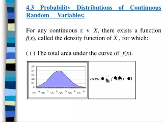
Continuous Density Functions Density functions, in contrast to mass functions, distribute probability continuously along an interval. The loading on the beam between points a & b is the integral of the function between points a & b. Figure 4-1 Density function as a loading on a long, thin beam. Most of the load occurs at the larger values of x. Sec 4-2 Probability Distributions & Probability Density Functions
A probability density function f(x) describes the probability distribution of a continuous random variable. It is analogous to the beam loading. Figure 4-2 Probability is determined from the area under f(x) from a to b. Sec 4-2 Probability Distributions & Probability Density Functions
Probability Density Function Sec 4-2 Probability Distributions & Probability Density Functions
Histograms A histogram is graphical display of data showing a series of adjacent rectangles. Each rectangle has a base which represents an interval of data values. The height of the rectangle creates an area which represents the relative frequency associated with the values included in the base. A continuous probability distribution f(x) is a model approximating a histogram. A bar has the same area of the integral of those limits. Figure 4-3 Histogram approximates a probability density function. Sec 4-2 Probability Distributions & Probability Density Functions
Area of a Point Sec 4-2 Probability Distributions & Probability Density Functions
Example 4-1: Electric Current Let the continuous random variable X denote the current measured in a thin copper wire in milliamperes (mA). Assume that the range of X is 0 ≤ x ≤ 20 and f(x) = 0.05. What is the probability that a current is less than 10mA? Answer: Figure 4-4 P(X < 10) illustrated. Sec 4-2 Probability Distributions & Probability Density Functions
Example 4-2: Hole Diameter Let the continuous random variable X denote the diameter of a hole drilled in a sheet metal component. The target diameter is 12.5 mm. Random disturbances to the process result in larger diameters. Historical data shows that the distribution of X can be modeled by f(x)= 20e-20(x-12.5), x ≥ 12.5 mm. If a part with a diameter larger than 12.60 mm is scrapped, what proportion of parts is scrapped? Answer: Sec 4-2 Probability Distributions & Probability Density Functions
Cumulative Distribution Functions Sec 4-3 Cumulative Distribution Functions
Example 4-3: Electric Current For the copper wire current measurement in Exercise 4-1, the cumulative distribution function (CDF) consists of three expressions to cover the entire real number line. Figure 4-6 This graph shows the CDF as a continuous function. Sec 4-3 Cumulative Distribution Functions
Example 4-4: Hole Diameter For the drilling operation in Example 4-2, F(x) consists of two expressions. This shows the proper notation. Figure 4-7 This graph shows F(x) as a continuous function. Sec 4-3 Cumulative Distribution Functions
Density vs. Cumulative Functions • The probability density function (PDF) is the derivative of the cumulative distribution function (CDF). • The cumulative distribution function (CDF) is the integral of the probability density function (PDF). Sec 4-3 Cumulative Distribution Functions
Exercise 4-5: Reaction Time • The time until a chemical reaction is complete (in milliseconds, ms) is approximated by this CDF: • What is the PDF? • What proportion of reactions is complete within 200 ms? Sec 4-3 Cumulative Distribution Functions
Mean & Variance Sec 4-4 Mean & Variance of a Continuous Random Variable
Example 4-6: Electric Current For the copper wire current measurement in Exercise 4-1, the PDF is f(x) = 0.05 for 0 ≤ x ≤ 20. Find the mean and variance. Sec 4-4 Mean & Variance of a Continuous Random Variable
Mean of a Function of a Random Variable Example 4-7: In Example 4-1, X is the current measured in mA. What is the expected value of the squared current? Sec 4-4 Mean & Variance of a Continuous Random Variable
Example 4-8: Hole Diameter For the drilling operation in Example 4-2, find the mean and variance of X using integration by parts. Recall that f(x) = 20e-20(x-12.5)dx for x ≥ 12.5. Sec 4-4 Mean & Variance of a Continuous Random Variable
Continuous Uniform Distribution • This is the simplest continuous distribution and analogous to its discrete counterpart. • A continuous random variable X with probability density function f(x) = 1 / (b-a) for a ≤ x ≤ b (4-6) Figure 4-8 Continuous uniform PDF Sec 4-5 Continuous Uniform Distribution
Mean & Variance • Mean & variance are: • Derivations are shown in the text. Be reminded that b2 - a2 = (b + a)(b - a) Sec 4-5 Continuous Uniform Distribution
Example 4-9: Uniform Current Let the continuous random variable X denote the current measured in a thin copper wire in mA. Recall that the PDF is F(x) = 0.05 for 0 ≤ x ≤ 20. What is the probability that the current measurement is between 5 & 10 mA? Figure 4-9 Sec 4-5 Continuous Uniform Distribution
Continuous Uniform CDF Figure 4-6 (again) Graph of the Cumulative Uniform CDF Sec 4-5 Continuous Uniform Distribution
Normal Distribution • The most widely used distribution is the normal distribution, also known as the Gaussian distribution. • Random variation of many physical measurements are normally distributed. • The location and spread of the normal are independently determined by mean (μ) and standard deviation (σ). Figure 4-10 Normal probability density functions Sec 4-6 Normal Distribution
Normal Probability Density Function Sec 4-6 Normal Distribution
Example 4-10: Normal Application Assume that the current measurements in a strip of wire follows a normal distribution with a mean of 10 mA & a variance of 4 mA2. Let X denote the current in mA. What is the probability that a measurement exceeds 13 mA? Figure 4-11 Graphical probability that X > 13 for a normal random variable with μ = 10 and σ2 = 4. Sec 4-6 Normal distribution
Empirical Rule P(μ – σ < X < μ + σ) = 0.6827 P(μ – 2σ < X < μ + 2σ) = 0.9545 P(μ – 3σ < X < μ + 3σ) = 0.9973 Figure 4-12 Probabilities associated with a normal distribution – well worth remembering to quickly estimate probabilities. Sec 4-6 Normal Distribution
Standard Normal Distribution A normal random variable with μ = 0 and σ2 = 1 Is called a standard normal random variable and is denoted as Z. The cumulative distribution function of a standard normal random variable is denoted as: Φ(z) = P(Z ≤ z) = F(z) Values are found in Appendix Table III and by using Excel and Minitab. Sec 4-6 Normal Distribution
Example 4-11: Standard Normal Distribution Assume Z is a standard normal random variable. Find P(Z ≤ 1.50). Answer: 0.93319 Find P(Z ≤ 1.53). Answer: 0.93699 Find P(Z ≤ 0.02). Answer: 0.50398 Figure 4-13 Standard normal PDF Sec 4-6 Normal Distribution
Example 4-12: Standard Normal Exercises • P(Z > 1.26) = 0.1038 • P(Z < -0.86) = 0.195 • P(Z > -1.37) = 0.915 • P(-1.25 < 0.37) = 0.5387 • P(Z ≤ -4.6) ≈ 0 • Find z for P(Z ≤ z) = 0.05, z = -1.65 • Find z for (-z < Z < z) = 0.99, z = 2.58 Figure 4-14 Graphical displays for standard normal distributions. Sec 4-6 Normal Distribution
Standardizing Sec 4-6 Normal Distribution
Example 4-14: Normally Distributed Current-1 From a previous example with μ = 10 and σ = 2 mA, what is the probability that the current measurement is between 9 and 11 mA? Answer: Figure 4-15 Standardizing a normal random variable. Sec 4-6 Normal Distribution
Example 4-14: Normally Distributed Current-2 Determine the value for which the probability that a current measurement is below this value is 0.98. Answer: Figure 4-16 Determining the value of x to meet a specified probability. Sec 4-6 Normal Distribution
Example 4-15: Signal Detection-1 Assume that in the detection of a digital signal, the background noise follows a normal distribution with μ = 0 volt and σ = 0.45 volt. The system assumes a signal 1 has been transmitted when the voltage exceeds 0.9. What is the probability of detecting a digital 1 when none was sent? Let the random variable N denote the voltage of noise. This probability can be described as the probability of a false detection. Sec 4-6 Normal Distribution
Example 4-15: Signal Detection-2 Determine the symmetric bounds about 0 that include 99% of all noise readings. We need to find x such that P(-x < N < x) = 0.99. Figure 4-17 Determining the value of x to meet a specified probability. Sec 4-6 Normal Distribution
Example 4-15: Signal Detection-3 Suppose that when a digital 1 signal is transmitted, the mean of the noise distribution shifts to 1.8 volts. What is the probability that a digital 1 is not detected? Let S denote the voltage when a digital 1 is transmitted. This probability can be interpreted as the probability of a missed signal. Sec 4-6 Normal Distribution
Example 4-16: Shaft Diameter-1 The diameter of the shaft is normally distributed with μ = 0.2508 inch and σ = 0.0005 inch. The specifications on the shaft are 0.2500 ± 0.0015 inch. What proportion of shafts conform to the specifications? Let X denote the shaft diameter in inches. Answer: Sec 4-6 Normal Distribution
Example 4-16: Shaft Diameter-2 Most of the nonconforming shafts are too large, because the process mean is near the upper specification limit. If the process is centered so that the process mean is equal to the target value, what proportion of the shafts will now conform? Answer: By centering the process, the yield increased from 91.924% to 99.730%, an increase of 7.806% Sec 4-6 Normal Distribution
Normal Approximations • The binomial and Poisson distributions become more bell-shaped and symmetric as their means increase. • For manual calculations, the normal approximation is practical – exact probabilities of the binomial and Poisson, with large means, require technology (Minitab, Excel). • The normal is a good approximation for the: • Binomial if np > 5 and n(1-p) > 5. • Poisson if λ > 5. Sec 4-7 Normal Approximation to the Binomial & Poisson Distributions
Normal Approximation to the Binomial Suppose we have a binomial distribution with n = 10 and p = 0.5. Its mean and standard deviation are 5.0 and 1.58 respectively. Draw the normal distribution over the binomial distribution. The areas of the normal approximate the areas of the bars of the binomial with a continuity correction. Figure 4-19 Overlaying the normal distribution upon a binomial with matched parameters. Sec 4-7 Normal Approximation to the Binomial & Poisson Distributions
Example 4-17: In a digital comm channel, assume that the number of bits received in error can be modeled by a binomial random variable. The probability that a bit is received in error is 10-5. If 16 million bits are transmitted, what is the probability that 150 or fewer errors occur? Let X denote the number of errors. Answer: Can only be evaluated with technology. Manually, we must use the normal approximation to the binomial. Sec 4-7 Normal Approximation to the Binomial & Poisson Distributions
Normal Approximation Method Sec 4-7 Normal Approximation to the Binomial & Poisson Distributions
Example 4-18: Applying the Approximation The digital comm problem in the previous example is solved using the normal approximation to the binomial as follows: Sec 4-7 Normal Approximation to the Binomial & Poisson Distributions
Example 4-19: Normal Approximation-1 Again consider the transmission of bits. To judge how well the normal approximation works, assume n = 50 bits are transmitted and the probability of an error is p = 0.1. The exact and approximated probabilities are: Sec 4-7 Normal Approximation to the Binomial & Poisson Distributions
Example 4-19: Normal Approximation-2 Sec 4-7 Normal Approximation to the Binomial & Poisson Distributions
Reason for the Approximation Limits The np > 5 and n(1-p) > 5 approximation rule is needed to keep the tails of the normal distribution from getting out-of-bounds. As the binomial mean approaches the endpoints of the range of x, the standard deviation must be small enough to prevent overrun. Figure 4-20 shows the asymmetric shape of the binomial when the approximation rule is not met. Figure 4-20 Binomial distribution is not symmetric as p gets near 0 or 1. Sec 4-7 Normal Approximation to the Binomial & Poisson Distributions
Normal Approximation to Hypergeometric Recall that the hypergeometric distribution is similar to the binomial such that p = K / N and when sample sizes are small relative to population size. Thus the normal can be used to approximate the hypergeometric distribution also. Sec 4-7 Normal Approximation to the Binomial & Poisson Distributions
Normal Approximation to the Poisson Sec 4-7 Normal Approximation to the Binomial & Poisson Distributions
Example 4-20: Normal Approximation to Poisson Assume that the number of asbestos particles in a square meter of dust on a surface follows a Poisson distribution with a mean of 100. If a square meter of dust is analyzed, what is the probability that 950 or fewer particles are found? Sec 4-7 Normal Approximation to the Binomial & Poisson Distributions
Exponential Distribution • The Poisson distribution defined a random variable as the number of flaws along a length of wire (flaws per mm). • The exponential distribution defines a random variable as the interval between flaws (mm’s between flaws – the inverse). Sec 4-8 Exponential Distribution