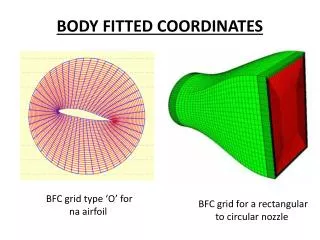
BODY FITTED COORDINATES
BODY FITTED COORDINATES. DOCUMENTATION. BFC phoenics online documentations: Introduction , Boundary Conditions and GCV (general colocated velocity method) Tutorials (look for BFC tutorials) Browse at the phoenics input library cases for: BFC and Multblock. When To Use BFCs.


BODY FITTED COORDINATES
E N D
Presentation Transcript
DOCUMENTATION • BFC phoenics online documentations: • Introduction, • Boundary Conditions and • GCV (general colocated velocity method) • Tutorials (look for BFC tutorials) • Browse at the phoenics input library cases for: BFC and Multblock
When To Use BFCs • BFCs are particularly suitable for internal or external flows with smoothly-varying non-regular boundaries. • For such flows, BFCs provide: • good geometric representation, • possibility of economical grid refinement close to the surface, • good representation of surface boundary layers, and hence of wall friction and heat transfer. • BFCs can also be used to reduce numerical "false-diffusion" errors, by aligning the grid with the local flow direction where possible, e.g., for angled jets (inclined fan heater in a room)
Coordinate Systems • Columns of cells must continue from one end of the grid to the other, i.e., the mesh is structured. • The cells are counted using the same conventions as in Cartesian and polar geometries: • 1 to NX in the IX-direction • 1 to NY in the IY-direction • 1 to NZ in the IZ-direction • The grid corner points must be prescribed by the user, via a Cartesian frame of axes, (XC, YC, ZC). • The alignment of the Cartesian axes - and the origin - can be chosen arbitrarily. • NOTE: The Cartesian coordinates (XC,YC,ZC) must NOT be confused with the cell-indices (IX,IY,IZ). • Note how the Cartesian and grid axes only coincide for the first few cells.
Structure of the Grid File • XC, YC and ZC are the Cartesian co-ordinates of the nodes. • Note that: I goes from West to East, J goes from South to North, and K goes from Low to High. • I, J & K count nodes (cell corners), • IX, IY & IZ count cells. • NX, NY and NZ are the numbers of cells in the I (IX), J (IY) & K (IZ) directions. WEST EAST I=6 I=1 IX=1 IX=5
Velocity Components IY • Q is the total velocity vector. • U1, V1 (and W1) are the SOLVEd velocity resolutes. • UCRT, VCRT (and WCRT) are the deduced vector components in the Cartesian coordinate system. • UC1, VC1 (and WC1) are the deduced vector components in the grid line directions (the co-located velocities) IX
The Steps In BFC Grid Generation • Specify POINTS - provide the Cartesian coordinates of key features of the geometry to be meshed • Specify LINES - join the points by lines, which are divided into segments corresponding to the number of cells which lie along the line. Lines may be straight, arc segments, or spline curves through defined points. • Create FRAMES - link the lines to make 2-D FRAMES. Frames always have four corners. • MATCH Grid to Frames - match the grid plane to appropriate frames. • Form the 3-D Grid - link 2-D grid planes to form a 3-D grid.
LINES POINTS EACH LINE IS DIVIDED IN POINTS WHICH WILL FORM THE VOLUMES FORMING THE FRAMES EACH FRAME HAS ALWAYS 4 CORNERS EXTRUDING TO FORM VOLUMES • SEE ADDITIONAL INFORMATION AT: Introduction,
WORKSHOP#1: SETTING A BFC GRID • Problem data 5 5 Y 5 10 X DIMENSION: NX = 15 & NY = 10 Set to view plane (XY); clickonmeshtogle; Select BFC grid
WORKSHOP#1 – STEP2Setting: points, lines, dimension and lines RESCUE Q1
WORKSHOP#1 – Step 3FRAMES always have 4 corners only Frame#1: corners Frame#2: corners Frame#3: corners Number of Cells on each side of the Frame has to match!
WORKSHOP#1 – Step 4 Match a grid Pick the first corner of a Frame Match the corner with the NODES coordinates Specify the first corner direction to the next points. All frames have right-handed axes. Ex: B->C +I & C->D +J (I,J,K) (1,6,1) (I,J,K) (1,1,1) (I,J,K) (6,1,1) RESCUE Q1
WORKSHOP#1 – Step 5 Volume Grid along (XY) plane To create volumes is necessary to extrude the grid along the K direction
Inlet Boundary Conditions • It is a special b.c. because the mass fluxes are related to the U1, V1, W1 resolute and not to the UCRT, VCRT and WCRT. • In general the required angles will vary from cell to cell. • Subroutine GXBFC has been provided to calculate the inlet conditions automatically, for the case of uniform inflow. • UCRT, VCRT, WCRT and density is non-standard, and simply provides a mechanism for transmission of UIN, VIN, WIN and RHOIN to GXBFC • SEE ADDITIONAL INFORMATION AT: Boundary Conditions
Use Of Cyclic Boundaries • The default setting in PHOENICS is no cyclic conditions, and a symmetry condition is assumed. • Cyclic (or periodicity) boundary conditions applies only along the east and west boundaries of XZ plane. • The provision for BFCs is intended for turbomachine (and airfoil) applications in which cyclic conditions are needed at the entrance to and exit from the blade passage. • To activate x-cyclic boundaries: Group 6, Q1 file: • XCYIZ(1,NZ,T) (switches XCYCLE on for all IZ slabs) • XCYIZ(1,9,T) (switches XCYCLE on for IZ=1 to 9) case B523 exemplifies the use of x-cyclic boundary conditions for the flow through a cascade of wedges
WORKSHOP#1: SET UP A CASE USING BFC plate inlet plate plate • Models: • elliptic GCV and, • solution for Vel & P • KECHEM • Numerics: 200 iter. • Props: Fluid: air(0) • Create objects: • inlet size: (10,1,1) & -2 m/s, • outlet size (5,1,1) • blocakge. • Note: case B116 has 15x15 volumes. outlet RESCUE Q1
Automatic Block Links • The GCV solver uses overlapping cells at block joints. These cells must exist in the individual block grid files. • Link automatic is when the blocks blocks share the same IJK orientation and same number of cells
A Natural Link • A natural link is when the blocks share the same IJK orientation but not the same number of cells B2 S • B1 share the north face of L3 with the south face of B2 N B1
Basic steps for Multi-Block Setup • Plan the decomposition of domain into individual blocks. A possible configuration is shown above. Block 1 is to be 5 x 15 x 1, and Block 2 is to be 15 x 5 x 1. • Generate the grid for each individual block. The grid for each block will be generated in a separate mesh-generator session. • Combine the grids to form the multi-block grid and define inter-block links. This step involves hand-editing the input Q1 file. • Define remainder of the problem (variables, boundary conditions, etc). B2 B1
Block links J=6 • The GCV solver uses overlapping cells at block joints. These cells must exist in the individual block grid files. • Only the linked faces of a block require an extra layer of dummy cells. • Block B1 has an extra plane of nodes at J =17 with thickness DY=0. • Similarly B2 has an extra plane of nodes at J = 1 with thickness DY =0 • These extra nodes are most conveniently copied exactly from the 'real' edge nodes, so that they are invisible to any viewing program. • See further examples at GCV B2 (15,6) J=2 J=1 J=17 DY=0 J=16 (16,5) B1 J=1
Linking the blocks in Q1 J=6 • TALK=T; • RUN( 1, 1) • BFC=T • NUMBLK=2 • READCO(GRI+) • MPATCH(1,MBL1-2, NORTH,1,NX,NY-1,NY-1,1,NZ,1,1) • MPATCH(2,MBL2-1, SOUTH,6,10,2,2,1,NZ,1,1) • STOP • See additional information on linking blocks atGCV B2 (15,6) J=2 J=1 J=17 DY=0 J=16 (16,5) B1 Y J=1 X
WORKSHOP#2 – Flow in a bifurcation; a natural link • Each block’s grid is developed and then linked together.
WORKSHOP#2 - Flow in a bifurcation; • We will follow the workshop on how to assemble natural links in a pipe bifurcation: wksh multiblock 1. • To short the drilling time, please download the q1 file which contains the Points and Lines. • After UPLOADING the file start from section: ‘Set grid for first block’ on wksh multiblock 1.
WORKSHOP#2 – Blocks’ construction; • Hint: before building MGRID2 (left) erase: the volume, the frame and the cells of MGRID1 (right) leaving only the lines. • Rescue q1 files at the links: MGRID1 and MGRID2.
WORKSHOP#2 – Assembling the case • Rescue q1 files at the links: MGRID3, GRI1, GRI2. Save these files at your working directory.
Unnatural Block Links • Link is unnatural when the blocks do not share the same IJK orientation B3 W N N S Blocks 1&2 and 1&3 are linked 'naturally' - West to East and South to north, whilst the link between 2&3 is 'unnatural' - a North face is linked to a West face. The instructions are in the tutorial: workshop multblock-2; also visit the links: READCO , MPATCH and link the three blocks. Y B2 W E B1 X
Basic steps for Multi-Block Setup Plan the decomposition of domain into individual blocks. A possible configuration is shown above. Each block is to be 5 x 5 x 1. Generate the grid for each individual block. The grid for each block will be generated in a separate mesh-generator session. Combine the grids to form the multi-block grid and define inter-block links. This step involves hand-editing the input Q1 file. Define remainder of the problem (variables, boundary conditions, etc).
WORKSHOP#3 - Flow in a disk sector; • We will follow the workshop on how to assemble un-natural links in a disk sector: workshop multblock-2 • To short the drilling time, please download the q1 file which contains the Points and Lines. • After UPLOADING the file start from section: ‘Set grid for first block’ on workshop multblock-2
WORKSHOP#3 – Blocks’ extrusion parameters B3 B2 B1 B3 B2 B1 BLOCK # B1 B2 B3 Length plane plane plane from/to from/to from/to Direction K 1 to 2 1 to 2 1 to 2 dZ = 1 Direction J 6 to 7 6 to 7 2 to 1 dY = 0 Direction I 2 to 1 6 to 7 2 to 1 dX = 0 UGRID3.q1 W UGRID1.q1 UGRID2.q1 N N E W S
WORKSHOP#3 - Matching Blocksq1 code lines TALK=T;RUN(1,1) BFC=T GCV=T NUMBLK=3 READCO(UGRI+) MPATCH(1,MBL1.2,WEST,2,2,1,NY-1,1,NZ,1,1) MPATCH(2,MBL2.1,EAST,NX-1,NX-1,1,NY-1,1,NZ,1,1) MPATCH(1,MBL1.3,NORTH,2,NX,NY-1,NY-1,1,NZ,1,1) MPATCH(3,MBL3.1,SOUTH,2,NX,2,2,1,NZ,1,1) MPATCH(2,MBL2.3,NORTH,1,NX-1,NY-1,NY-1,1,NZ,1,1) MPATCH(3,MBL3.2,WEST,2,2,2,NY,1,NZ,1,1) SPEDAT(SET,GCV,MBL3.2,C,WNL) STOP B3 B2 B1 • If the blocks are rotated relative to each other in IJK space (B3 to B2), the block alignment must be specified through SPEDAT command. • This string defines how the N, E and H faces of the first block link to the second block. The default, natural, link would be S W L; i.e. North to South, East to West and High to Low, see B1 to B3 and B2 to B1. W N N E W S
WORKSHOP#3 - SPEDAT COMMAND & BLOCK ROTATION B3 is rotated 90º from B2 B3 Blocks’ Linkages B3 y x B2 B2 B3 y B1 x BLOCK#3 -> N E H BLOCK#2 -> W N L SPEDAT(SET,GCV,MBL3.2,C,WNL) W W The string defining the block rotation consists of three letters, which may be any of E W N S H L. The individual characters define the relative orientation between the N, Eand H faces of the first block (B2) of the pair of blocks, and the current block (B3) respectively. N N N N N E E W W W E E S S S S
WORKSHOP#3 – Case setting; • Properties: air (0) • Model: laminar, activatevelocities, CGV • Numerics: 100 iteractions • Objectcs: Inlet (V = 1,0 m/s) & Outlet
WORKSHOP#3 – Results • Rescue q1 files at the links: UGRID123, UGRI1, UGRI2, UGRI3. Save these files at your working directory.
Multblock Application in Complex Geometry • The selected figures come from the cases available in the phoenics input library ( Multiblock)
Phoenics BFC Generator • The Phoenics built-in BFC Generator is helpful for simple problems. • If one application demands several ‘natural or unnatural’ links the mesh generation process becomes very complex. • In this scneario phoenics BFC generator is not recommended. There are specific software for mesh generation recommended such as: ICEM,
Airfoil Grids http://courses.cit.cornell.edu/fluent/airfoil/step1.htm • The domain size is expressed in terms of the airfoil thickness. • Airfoil with finite thickness (present illustration) require Natural and/or Unnatural links, unfortunately. It is not an easy task to do using Phoenics BFC grid generator!
C Grids for FiniteThicknesAirfoil( represent the frames’ corners) zero thickness trailing edge B3 • Blocks B1, B2, B3 have natural links • B4 is 180o rotated in regard to B1. • Multi Block grid. • Provide extra Y cells to B1 and B4 • SPEDAT(SET,GCV,MBL4.1,C,NEL) B4 B1 B2 (F) (E) (G) (F) (E) (D) (G) finite thickness trailing edge (L) B4 B3 • Blocks B1, B2, B4 have natural links • B3 is 180o rotated in regard to B4. • Multi Block grid. • Provide extra Y cells to B4 and B3 • SPEDAT(SET,GCV,MBL4.3,C,NEL) (D) (L) (H) (A) (B) (C) B1 y y y y B2 x x x x (A) (B) (C)
Finite x Small Thickness Airfoil • The small thickness airfoil is gives an approximated solution. • The thin airfoil consists of a line and it is easily setup on the BFC mesh generator in phoenics.
Natural links for airfoil: grid This grid would be a 2nd choice for the C grid. It still can be improved by changing the inclination of lines L23 & L24 an designing a better number of cells to result in a more orthogonal mesh. One can also design a similar grid for a zero thickness airfoil