Flow shop production
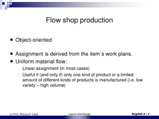
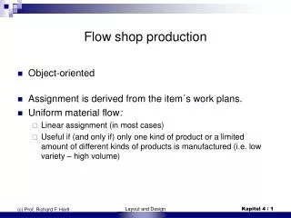
Flow shop production. Object-oriented Assignment is derived from the item´s work plans. Uniform material flow : Linear assignment (in most cases)

Flow shop production
E N D
Presentation Transcript
Flow shop production • Object-oriented • Assignment is derived from the item´s work plans. • Uniform material flow: • Linear assignment (in most cases) • Useful if (and only if) only one kind of product or a limited amount of different kinds of products is manufactured (i.e. low variety – high volume) Layout and Design
Flow shop production According to time-dependencies we distinguish between • Flow shop production without fixed time restriction for each workstation („Reihenfertigung“) • Flow shop prodcution with fixed time restriction for each workstation (Assemly line balancing, „Fließbandabgleich“) Layout and Design
Flow shop production • No fixed time restriction for the workload of each workstation: • Intermediate inventories are needed • Material flow should be similiar for all prodcuts • Some workstations may be skipped, but going back to a previous department is not possible • Processing times may differ between products Layout and Design
Flow shop production • Fixed time restricition (for each workstation): • Balancing problems • Cycle time („Taktzeit“): upper bound for the workload of each workstation. • Idle time: if the workload of a station is smaller than the cycle time. • Production lines, assembly lines • automated system (simultaneous shifting) Layout and Design
Assembly line balancing • Production rate = Reciprocal of cycle time • The line proceeds continuously. • Workers proceed within their station parallel with their workpiece until it reaches the end of the station; afterwards they return to the begin of the station. • Further possibilites: • Line stops during processing time • Intermittent transport: workpieces are transported between the stations. Layout and Design
Assembly line balancing • „Fließbandabstimmung“, „Fließbandaustaktung“, „Leistungsabstimmung“, „Bandabgleich“ • The mulit-level production process is decomomposed into n operations/tasks for each product. • Processing time tjfor each operation j • Restrictions due to production sequence of precedences may occur and are displayed using a precedence graph: • Directed graph witout cyles G = (V, E, t) • No parallel arcs or loops • Relation i< j is true for all (i, j) Layout and Design
Example Precedence graph Layout and Design
Flow shop production • Machines (workstations) are assigned in a row, each station containing 1 or more operations/tasks. • Each operation is assigned to exactly 1 station • I before j – (i, j) E: • i and j in same station or • i in an earlier station than j • Assignment of operations to staions: • Time- or cost oriented objective function • Precedence conditions • Optimize cycle time • Simultaneous determination of number of stations and cycle time Layout and Design
Single product problems • Simple assembly line balancing problem • Basic model with alternative objectives Layout and Design
Single product problems Assumptions: • 1 homogenuous product is produced by performing n operations • given processing times ti for operations j = 1,...,n • Precedence graph • Same cycle time for all stations • fixed starting rate („Anstoßrate“) • all stations are equally equipped (workers and utilities) • no parallel stations • closed stations • workpieces are attached to the line Layout and Design
Alternative1 Minimization of number of stationsm (cycle time is given): Cycle time c: • lower bound for number of stations • upper bound for number of stations Layout and Design
Alternative 1 t(Sk) … workload of station kSk, k = 1, ..., m Integer property Sum of inequalities and integer property of m tmax + t(Sk) > c i.e. t(Sk) c + 1 - tmaxk =1,...,m-1 upper bound Layout and Design
Alternative 2 Minimization of cycle time (i.e. maximization of prodcution rate) lower bound for cycle time c: • tmax =max {tj j = 1, ... , n} … processing time of longest operation ctmax • Maximum production amount qmaxin time horizon T is given • Given number of stations m Layout and Design
Alternative 2 • lower bound for cycle time: • upper bound for cycle time Layout and Design
Alternative 3 Maximization of efficiency („Bandwirkungsgrad“) • Determination of: • Cycle time c • Number of stations m Efficiency („BG“) • BG = 1 100% efficiency (no idle time) Layout and Design
Alternative 3 • Lower bound for cycle time: see Alternative 2 • Upper bound for cycle time cmax is given • Lower bound for number of stations • Upper bound for number of stations Layout and Design
ExampIe • T = 7,5 hours • Minimum production amount qmin = 600 units • seconds/unit Layout and Design
ExampIe tj = 55 No maximum production amount Minimum cycle timecmin = tmax = 10 seconds/unit Layout and Design
ExampIe Combinations of m and c leading to feasible solutions. Layout and Design
ExampIe • maximum BG = 1(is reached only with invalid values m = 1 and c = 55) • Optimal BG = 0,982(feasible values for m and c: 10 c45 und m 2) m = 2 stations c = 28 seconds/unit Layout and Design
Example Possible cycle times c for varying number of stations m Increasing cycle time Reduction of BG (increasing idle time) until 1 station can be omitted. BG has a local maximum for each number of stations m with the minimum cycle time c where a feasible solution for m exists. Layout and Design
Further objectives Maximization of BG is equivalent to • Minimization of total processing time („Durchlaufzeit“): D = m c • Minimization of sum of idle times: • Minimization of ratio of idle time: LA = = 1 – BG • Minimization of total waiting time: Layout and Design
LP formulation We distinguish between: • LP-Formulation for given cycle time • LP-Formulation for given number of stations • Mathematical formulation for maximization of efficiency Layout and Design
LP formulation for given cycle time • Binary variables: • = number of station, where operation j is assigned to • Assumption: Graph G has only 1 sink, which is node n j = 1, ..., n k = 1, ..., mmax Layout and Design
LP formulation for given cycle time Objective function: Constraints: • j = 1, ... , n ... j on exactly 1 station • k = 1, ... , mmax ... Cycle time • ... Precedence cond. • • ... Binary variables j and k Layout and Design
Notes Possible extensions: • Assignment restrictions (for utilities or positions) • elimination of variables or fix them to 0 • Restrictions according to operations • Operations h and j with (h, j) are not allowed to be assigned to the same station. Layout and Design
LP formulation for given number of stations • Replace mmax by the given number of stations m • c becomes an additional variable Layout and Design
LP formulation for given number of stations Objective function: Minimize Z(x, c) = c … cycle time Constraints: j = 1, ... , n ...j on exactly 1 station k = 1, ... , m ... cycle time ... precedence cond. j und k ... binary variables c 0 integer Layout and Design
LP formulation for maximization of BG • If neither cycle time c nor number of stations m is given take the formulation for given cycle time. Objective function (nonlinear): Additional constraints:c cmax c cmin Layout and Design
LP formulation for maximization of BG • Derive a LP again Weight cycle time and number of stations with factors w1 and w2 Objective function (linear): Minimize Z(x,c) = w1(kxnk) + w2c Large Lp-models! Many binary variables! Layout and Design
Heuristic methods in case of given cycle time • Many heuristic methods(mostly priorityrule methods) • Shortened exact methods • Enumerative methods Layout and Design
Priorityrule methods • Determine a priortity value PVj for each operations j • Prioritiy list • A non-assigned operation j can be assigned to station k if • all his precedessors are already assigned to a station 1,..k and • the remaining idle time in station k is equal or larger than the processing time of operation j. Layout and Design
Priorityrule methods • Requirements: • Cycle time c • Operations j=1,...,n with processing times tj c • Precedence graph, defined by a sets of precedessors. • Variables • k number of current station • idle time of current station • Lp set of already assigned operations • Ls sorted list of n operations in respect to priority value Layout and Design
Priorityrule methods • Operation j Lp can be assigned, if tjand h Lp is true for all h V(j) • Start with station 1 and fill one station after the other • From the list of operations ready to be assigned to the current station the highest prioritized is taken • Open a new station if the current station is filled to the maximum Layout and Design
Priorityrule methods Start: determine list Ls by applying a prioritiy rule; k := 0; LP := <]; ... No operations assigned so far Iteration: repeat k := k+1; := c; while there is an operation in list Ls that can be assigned to station k do begin select and delete the first operation j (that can be assigned to) from list Ls; Lp:= < Lp,j]; :=- tj end; untilLs= <]; Result:Lp contains a valid sorted list of operations with m = k stations. Single-pass- vs. multi-pass-heuristics(procedure is performed once or several times) Layout and Design
Priorityrule methods • Rule 1: Random choice of operations • Rule 2: Choose operations due to monotonuously decreasing (or increasing) processing time: PVj: = tj • Rule 3: Choose operations due to monotonuously decreasing (or increasing) number of direct followers: PVj : = (j) • Rule 4: Choose operations due to monotonuously increasing depths of operations in G:PVj : = number of arcs in the longest way from a source of the graph to j Layout and Design
Priorityrule methods • Rule 5 Choose operations due to monotonuously decreasing positional weight („Positionswert“): • Rule 6: Choose operations due to monotonuously increasing upper bound for the minimum number of stations needed for j and all it´s predecessors:: • Rule 7: Choose operations due to monotonuously increasing upper bound for the latest possible station of j: Layout and Design