
Image Processing & Antialiasing
Image Processing & Antialiasing. Part II (Aliasing, Sampling, Convolution, and Filtering). Outline. Overview Example Applications Jaggies & Aliasing Sampling & Duals Convolution. Filtering Scaling Reconstruction Scaling, continued Implementation. Jaggies & Aliasing.
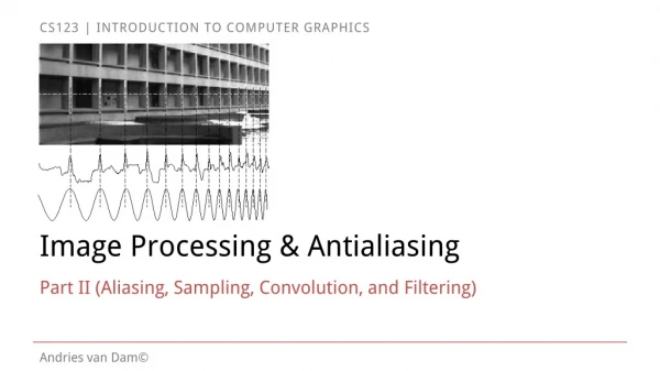

Image Processing & Antialiasing
E N D
Presentation Transcript
Image Processing & Antialiasing Part II (Aliasing, Sampling, Convolution, and Filtering)
Outline 9/24/19 Overview Example Applications Jaggies & Aliasing Sampling & Duals Convolution Filtering Scaling Reconstruction Scaling, continued Implementation
Jaggies & Aliasing • “Jaggies” is an informal name for artifacts caused by poorly representing continuous geometry by a discrete 2D grid of pixels – a form of aliasing (later…) • Jaggies are a manifestation of sampling error and loss of information (aliasing of high frequency components by low frequency ones) • Effect of jaggies can be reduced by anti-aliasing, which smoothes out the pixels around the jaggies by averaging • Shades of gray instead of sharp black/white transitions • Diminishes HVS’ “edge detection” response to sharp transitions (Mach banding) 9/24/19
In the ‘80s, we knew about aliases...but not enough about anti-aliasing https://youtu.be/TpDuxfA4DOI demo Related phenomenon: Moire patterns 9/24/19 So we blithely blurred a rendered (relatively low-rez) image and it did look a bit better… Until we made an animation of the CIT model projected on a 20ft screen hung on the SciLi and were horrified by the “crawlies”: And we also did image scaling and were not happy with the results… We lacked a basic understanding of the theory behind filtering Let’s start with simpler problem than image scaling: rendering lines
Representing lines: Point sampling, single pixel • Midpoint algorithm: in each column, pick the pixel with the closest center to the line • A form of point sampling: sample the line at each of the integer X values • Pick a single pixel to represent the line’s intensity, full on or full off • Doubling resolution in x and y only lessens the problem, but costs 4 times memory, bandwidth, and scan conversion (rasterization) time! • Note: This works for -1 < slope < 1, use rows instead of columns for the other case or there will be gaps in the line Line approximation using point sampling Approximating same line at 2x the resolution 9/24/19
Representing lines: Area sampling • Represent the line as a unit width rectangle, use multiple pixels overlapping the rectangle (for now we think of display pixels as squares) • Instead of full on/off, calculate each pixel intensity proportional to the area covered by the unit rectangle • A form of “unweighted area sampling” – stay tuned: • Only pixels covered by primitive can contribute • Distance of pixel center to line doesn’t matter • Typically have more than one pixel per column so can go more gradually from dark for pixels covered by the line to white background; the more area of overlap, the darker the pixel 9/24/19
Filtering as form of averaging: a filter is a weighting function • Apply an unweighted or weighted average to each sample and its neighbors to decrease contrast, make graph look smoother • Example: filtering for student height – give each sample equal weight or diminish influence of samples further away • The weight function used above gives different weight to each sample around x • The area of the weight function needs to be 1 to preserve overall brightness Weight function = centered at some value of x, often a pixel center Pre-Filtered samples Post-filtered samples (decreases contrast between adjacent pixels): red = weighted value 9/24/19
“Box Filter” Represents Unweighted Area Sampling • Box filter is constant over all area and is a single pixel wide here, but could vary in width • For each pixel intersecting the line, the intensity contributed by each infinitesimal area of the line is • The total intensity of the pixel (between 0 and 1) integrated over area of overlap is: • Integral is volume over area of overlap (in above figure, a rectangular wedge) 9/24/19
“Cone Filter” for Weighted Area Sampling • Area sampling, but the overlap between filter and primitive is weighted so that sub-areas with closer to center of pixel count more • Cone has: • Linear falloff • Circular symmetry • Width of 2 (called support) • Intensity of pixel is the “subvolume” inside the cone over the line (see picture) 9/24/19
2-unit circular support of filter Weighted Area Sampling (Continued) Pixel center (+) W Area of overlap between support and primitive Differential area dA1 Differential area dA2 Primitive 9/24/19 W is the weight which is multiplied with at ; normalize Wto make volume under cone = 1
Another Look at Point Sampling – Even Box Filter is Better! • This simplistic scan conversion algorithm only asks if a mathematical point is inside the primitive or not • Bad for sub-pixel detail which is very common in high-quality rendering where there may be many more micro-polygons than pixels! A C D B Point-sampling problems. Samples are shown as black dots. Object A and C are sampled, but corresponding objects B and D are not. 9/24/19
Another Look at Unweighted Area Sampling: Box filter • Box filter • Support: 1 pixel • Sets intensity proportional to area of overlap • Creates “winking” of adjacent pixels as a small triangle translates (b) Unweighted area sampling. (a) All sub-areas in the pixel are weighted equally. (b) Changes in computed intensities as an object moves between pixels. 9/24/19
Another Look at Weighted Area Sampling: Cone filter • Cone filter • Support: 2 pixels • Greater smoothness in the changes of intensity (b) Weighted area sampling with overlap. (a) Typical weighting function. (b) Changes in computed intensities as an object moves between pixels. 9/24/19
Pseudocode and Results for each sample point p: //p need not be integer! place filter centered over p for each pixel q under filter: weight = filter value over q p.intensity += weight * q.intensity Filter Shapes for Image Scaling Demo 9/24/19 Aliased Anti-aliased
Anti-Aliasing Example Close-up of original, aliased render Antialiasing Techniques: Blur filter – weighted average of neighboring pixels Supersampling - sample multiple points within a given pixel and average the result Checkerboard with Supersampling Supersampling and Blurring 9/24/19
In – Class Question 1 9/24/19
Outline 9/24/19 Overview Example Applications Jaggies & Aliasing Sampling & Duals Convolution Filtering Scaling Reconstruction Scaling, continued Implementation
Aliasing and Anti-Aliasing: Intro to Signal Processing • Easier to discuss aliasing and anti-aliasing of images and image scaling than of rendering anti-aliased geometric primitives - return to rendering primitives at end of this unit • A signal is a time- or spatially varying function (sound wave, brightness of an image, electromagnetic wave…): • “A signal is a physical quantity that varies with time, space, or any other independent variable by which information can be conveyed“ – from WikiBooks entry on signals (think turn signal, umpire’s signal, body language…) • Need to do a brief intro to signal processing, since an image can be thought of as a sequence of scan lines, each displaying an intensity signal • Core concept: signals are often complex-looking functions but they can be decomposed into combinations of simpler functions (sines and cosines) of varying frequency, amplitude and phase – compare to decomposing vectors • Fourier Analysis/Synthesis 9/24/19
Sampling and Scaling of Images(images courtesy of George Wolburg, Columbia University, in 2nd Edition Computer Graphics: P&P) • Scan converting an image is digitizing (sampling) a series of continuous intensity functions, one per scan line – each is a signal • We will use single scan lines for simplicity, but everything still applies to full images Scan line from synthetic scene Scan line from natural scene (the real world or a high-rez photo) 9/24/19
The Sampling/Reconstruction/Display Pipeline – overview Original continuous signal: Sampled signal (lose information): Reconstructed signal (approximation to original): (many reconstruction methods) One (poor but simple) reconstruction method is linear interpolation of samples: 9/24/19
Fourier Waveform Synthesis – Approximate a Continuous Signal Approximation of scan line signal from image improves with addition of a sequence of sine waves of higher frequency but lower amplitude • Any signal can be approximated by summing sine (and cosine) waves of different frequencies, phases, and amplitudes 9/24/19
Digression: Music • A vibrating string creates a pressure wave with multiple frequency components • Intensity/volume of sound is related to amplitudes of components of pressure wave • Lowest frequency is “fundamental frequency” Labels show 1/f -- the wavelength • Integer multiples of the fundamental frequency are called “harmonics” or “overtones” (non-integral multiples also exist) • Power of two multiples of the fundamental frequency are called “octaves” An applet to interact with these concepts: https://phet.colorado.edu/en/simulation/fourier 9/24/19
Analogous Operations, Duals (1/2) • A signal has 2 representations. We’re familiar with the spatial domain, but every signal also can be represented in the frequencydomain • Spatial and frequency domains are duals and represent identical information, as we shall see • Easier to visualize signals and filtering/averaging in the frequency domain (see S25) • Characterize a signal by its frequency spectrum showing amplitudes of component sin (and/or cos) waveforms • Easier to understand filtering in frequency domain than in signal domain, as we shall see shortly • Many problems are easier solved by transforming to another, related, problem 9/24/19
Analogous Operations, Duals (2/2) • Take a familiar problem: multiplication of numbers • Can take logarithm of number, perform operations on log(number), then take antilogarithm) • Dual of multiplication is addition in logarithmic “dual” If ab=c then log(a) + log(b) = log(c) • This “invertible transformation” makes slide-rules such effective tools for multiplication: manipulating sliders corresponds to manipulating numbers via their logs • To multiply, add lengths of number on slider and on fixed rule as logs, then read antilog under cursor 9/24/19
Frequency Spectrum of a Signal Signal Domain Frequency Domain • Sine wave is characterized by amplitude and frequency • Frequency of a sine wave is number of intensity cycles per second for audio, or number of brightness cycles per unit length (e.g., inter-pixel distance) for image scan lines • Can characterize any waveform by enumerating amplitude and frequency of all its component sine waves (Fourier transform – see chapter 18 in book) • This can be plotted as a “frequency spectrum”, a.k.a. power spectrum, (we ignore negative frequencies, but they are needed for mathematical correctness) To see spatial and frequency domains of simple signals see Evan Wallace’s demo. By taking a subset of the frequency spectrum get an approximate reconstruction of the original signal https://xkcd.com/26/ 9/24/19
Sine waves in 2D • Let white be max positive amplitude, black max negative amplitude Higher Frequency (Harmonic – integer multiple) Low Frequency Images from http://cns-alumni.bu.edu/~slehar/fourier/fourier.html 9/24/19 Images: Hays
Simple Fourier Synthesis example (1/2) • example : g(t) = sin(2πf t) + (1/3)sin(2π(3f) t) + = 9/24/19 Slides: Hays
Simple Fourier Synthesis example (2/2) • Approximate signal using sines and cosines Partial approximation with 4 cosines (red and green) Spatial domain Original Function Partial approximation with 2 cosines Partial approximation with 3 cosines Approximation with 5 cosines f(x) We are just summing waves to get bolded blue function to approximate the red signal x 9/24/19
Sampling: The Nyquist Limit • In order to capture all frequencies in a signal, we must sample at a rate that is higher than 2 times the highest frequency (with a non-zero value from the Fourier transformation) in the signal (the Nyquist limit). • Here is an approximate analog sine wave: • The sine wave sampled at an acceptable rate (4 times the highest frequency): • Reconstructed wave based on these samples (draw a nice smooth curve thru or near sample points): Digression: Pixar Article 9/24/19
Aliasing: Know Thine Enemy • Aliasing occurs when we sample a signal at less than twice maximum frequency • Here is our analog sine wave again: • Here is the sine wave sampled at too low a rate: • Here is the reconstructed wave based on these samples: • The reconstruction isn’t even close! 9/24/19
Temporal Aliasing: Another Sampling Error • Ever seen tires spin in a movie? Have you ever noticed that sometimes, they seem to be spinning backwards? • It’s because the video frame-rate is lower than twice the frequency at which the wheels spin. This is temporal aliasing! • You see this a lot in movies because the effect is so striking.It’s known as the stage-coacheffect. • Porsche Dyno Test 9/24/19
Sampling at the Nyquist Limit • Sampling right at the Nyquist limit can also be problematic • Here is our perfect analog sine wave again: • Here is the sine wave sampled at the Nyquist limit. This time it works fine: • Here is the same sine wave sampled at the Nyquist limit, with the sample points shifted. Now we get no signal: • For an applet dedicated to illustrating the Nyquist Limit: Nyquist Limit Demo 9/24/19
The Enemy is Recognized • Aliasing is shown in bottom diagrams on previous slides – signals that are sampled at too low a rate can reconstruct high frequencies as low frequencies • These low frequencies are “aliases” of high frequencies • The low sampling rate data could not adequately represent the high frequency components, so it represented them incorrectly, as low frequencies • So, we just sample above the Nyquist limit, right? • Regrettably, we can’t always do that • What about this square wave signal? Just a test pattern of alternating black/white bars • Let’s try using Fourier Synthesis Number of sine waves 9/24/19 125 25 5
Infinite Frequencies • Square waves have infinite frequencies at the jumps, so how can we sample correctly at those edges? • We can’t. Pure and simple. , and we can’t sample at an infinite rate. • Unfortunately, infinite frequencies are the rule in synthetic computer graphics - discrete transitions between adjacent pixels • So, do inverse operation. Instead of increasing our sampling frequency to meet that of the signal, we: • Pre-filter out high frequencies we can’t show • The signal is now guaranteed to consist only of frequencies we can represent and reconstruct with reasonable accuracy • This isn’t the same signal that came in, but it’s better than an aliased version • Reconstructing the pre-filtered approximate signal beats reconstructing sampled original signal, with its corrupting aliases for the highest frequencies 9/24/19
In-Class Question 2 9/24/19
Low-Pass to EliminateHigh Frequencies (shown for one scan line in Spatial Domain) 9/24/19
Ideal Low-Pass Filtering (Frequency Domain) • Multiplying by the box function in the frequency domain • Frequencies under the box are kept, and the high frequencies are cut off • Corresponds to convolution with the sinc function in the spatial domain (stay tuned) … … 9/24/19
Infinite Frequencies • The more high frequencies we pre-filter out, the lower the sampling frequency needed but the less the filtered signal resembles original. • Note: pre-filtering is often just abbreviated as filtering, but the prefix “pre” helps remind us that post-filtering (i.e., another stage of filtering after image computation or transformation) is also practiced. If post-filtering is done on reconstruction of samples of original signal, it will blur in the aliases present in the corrupted reconstruction! 9/24/19
Scale Aliasing, or “Why do we have to pre-filter?” This doesn’t look right at all. There are no stripes and the image now has a blacker average intensity Image with sample points marked Image scaled using point samples Original Image 9/24/19
Scale Aliasing II, or “Close, but no cigar?” Better, but not perfect… Prefiltered image with samples marked Prefiltered image scaled Original Image 9/24/19
Scale Aliasing III, or “Why is it still wrong?” • Good: The pre-filtered scaled image now has same overall brightness • Bad: still no stripes • Filter removed “high frequencies” from image • Discontinuities that were stripes • Given number of points to represent image once scaled, not enough points to represent high frequencies; even higher sampling rate doesn’t help… • Nyquist limit says that we can’t represent frequencies higher than ½ our sampling rate, thus can’t do better than this blurred approximation 9/24/19
Outline 9/24/19 Overview Example Applications Jaggies & Aliasing Sampling & Duals Convolution Filtering Scaling Reconstruction Scaling, continued Implementation
Filtering as an Application of the Convolution Integral • Remember filtering is just (weighted) averaging of samples in a neighborhood • How is it done in practice? Just a nested for loop through all the sample points • Either sample at integer pixel locations or in between (e.g., for image up-scaling) • Based on the theory of signal convolution – the convolution integral • We’ll use a finite approximation to that integral 9/24/19
Discrete convolution – Function as an Array • This is the type of convolution we will be using once we begin coding • Think of it as a fancy kind of multiplication • If we evenly sample a function, get an array of point samples, e.g., (R,G, B) triples as color intensity values • Some mathematicians think of an array of numbers as a function. Think this way for the next few slides! • The larger the array (the more samples/unit interval) the more accurate the representation of the original function and the better our ability to anti-alias and improve the reconstruction [ 1.2, 0, -1.2, 0, 1.2, 0, -1.2 ] 9/24/19
Discrete Convolution for Filtering • Have two arrays (functions), f and g, and we assign g as our “filter”. For the sake of convenience, force the filter to have an odd number of points so that there is a center • Once we are done with our convolution, we will produce a new array (function) • You’ll do this for the filter assignment for blur and edge detection, as well as for image scaling • Take the filter, and line up the center point of the filter with each element, i, of f. To do a weighted sum, multiply each pair of elements and sum the products. Assign this value to element i of the output array • When we are scaling, this procedure will change slightly because where we center the filter and where our value goes will be different! • One hiccup: The output array will be slightly larger than our initial array because we start our multiplication/sum process at the edges, where it will generate a non-zero result • It is easier to see! 9/24/19
Discrete Convolution – Visually (1/2) [ ⅓, ⅓, ⅓] [ 1.2, 0, -1.2, 0, 1.2, 0, -1.2 ] Function, f Function, g, a box filter (unweighted area sampling) 9/24/19
Discrete Convolution – Visually (2/2) [ 1.2, 0, -1.2, 0, 1.2, 0, -1.2 ] .4 [ .4, _, _, _, _, _, _ ] [ ⅓, ⅓, ⅓ ] [ 1.2, 0, -1.2, 0, 1.2, 0, -1.2 ] [ .4, .4, _, _, _, _, _ ] [ ⅓, ⅓, ⅓] [ 1.2, 0, -1.2, 0, 1.2, 0, -1.2 ] [ .4, .4, 0, _, _, _, _ ] [ ⅓, ⅓, ⅓ ] 0.0 [ 1.2, 0, -1.2, 0, 1.2, 0, -1.2 ] [ .4, .4, 0, -.4, _, _, _ ] [ ⅓, ⅓, ⅓ ] -.4 9/24/19
Discrete Convolution – Demo • Our demo shows this in practice 9/24/19
In-Class Question 3 9/24/19
Discrete Convolution – Review • Think of an array as a function • We take two arrays and generate a third • We “slide” the filter along the other array and at each element, calculate a value by multiplying the pairs and summing the products to do the (weighted) averaging • Our output array will be slightly larger than our input array if we start too far over the edges. We can (and will) ignore this for image processing and just take “inner” part of the array • Another hiccup: Our process has an additional step if our filter is not symmetric, but in this course filters will be symmetric 9/24/19


